
Tensors and Gradients in PyTorch
In this notebook we will learn what tensors are, why they are used and how to create and manipulate them in PyTorch.
Tensors
0D Tensor - Scalar
A 0-dimensional tensor, i.e. rank 0, is a simple scalar, i.e. a number, such as 42.
Rank in tensors represents the number of axes. In the case of a scalar, there are no axes and so rank is 0.
1D Tensor - Vector
A 1-dimensional tensor, rank 1 (one axis), is a vector which can in turn be n-dimensional, $n \in \mathbb{R^+}$.
For example, [20], [8,20], [92, 101, 200] are one-dimensional, two-dimensional and three-dimensional vectors respectively. All of these are examples of a 1D tensor.
2D Tensor - Matrix
A 2-dimensional tensor, rank 2 (two axes), is a matrix, $n \times m$, where $n,m \in \mathbb{R^+}$. For example, the following matrices, a $3 \times 4$ matrix and a $n \times m$ matrix respectively, are both 2D tensors.
\[\begin{bmatrix} 10 & 7 & 18 & 4 \\ 8 & 19 & 43 & 7 \\ 17 & 5 & 9 & 23 \\ \end{bmatrix}\] \[\begin{bmatrix} a_{11} & a_{12} & \cdots & a_{1m} \\ a_{21} & a_{22} & \cdots & a_{2m} \\ \vdots & \vdots & \ddots & \vdots \\ a_{n1} & a_{n2} & \cdots & a_{nm} \\ \end{bmatrix}\]3D Tensor
A 3-dimensional tensor, rank 3 (three axes), can be thought of as a vector of matrices.
Higher-order Tensors
To understand higher-order tensors, it is helpful to understand how 0D tensors up to 3D tensors fit together. A 0D tensor is just a scalar. A 1D tensor is a vector of scalars. In turn, a 2D tensor is a vector of vectors of scalars. Finally, a 3D tensor is a vector of vectors of vectors of scalars.
Following this pattern, higher-order tensors, such as a 4D tensor would pack one or more 3D tensors inside of it. In other words, a 4D tensor is a vector containing one or more 3D tensors. Taking this to the next level, a 5D tensor is in turn a vector containing one or more 4D tensors in it. This pattern carries on for further higher-order tensors. As you can see, visualising and imagining in our mind these higher order tensors becomes increasingly difficult, if not outright impossible.
What Do Tensors Represent in Practice?
A 0D tensor stores a scalar value, which could be anything really, say a regression value.
A 1D tensor stores a vector of values, say one training sample composed of $n$ features.
A 2D tensor stores a matrix of values, typically having a shape of $n\ samples \times m\ features$.
A 3D tensor is a vector of matrices of values, typically having a shape of $n\ samples \times t\ steps \times m\ features$. 3D tensors are typically used when storing time-series data or when sequence order is important, say text.
A 4D tensor is a vector of 3D tensors and is typically used to store image data. Each colour image has a width and a height, plus normally three colour channels. Thus each image is a 3D tensor of shape $height \times width \times channels$. Thus an images training batch is a 4D tensor, i.e. a vector of $n$ samples of 3D tensors.
Note : In TensorFlow, 4D image tensors have shape $N \times H \times W \times C$, channel-last convention. In constrast, in PyTorch, 4D image tensors have shape $N \times C \times H \times W$, channel-first convention.
A 5D tensor is in practice used to store batches of $n$ sample videos. Each video is a sequence of frames, i.e. images and so a 4D tensor has shape $frames \times height \times width \times channels$. Shape of 4D tensor might vary depending whether we are using channel-first $N \times C \times H \times W$ or channel-last $N \times H \times W \times C$ convention. In turn, the 5D tensor is a vector of $n$ sample videos, each a 4D tensor.
Creating Tensors in PyTorch
Importing Libraries
import torch
import numpy as np
import pandas as pd
import matplotlib.pyplot as plt
Support Functions
def tensor_properties(t, show_value=True):
    print('Tensor properties:')
    props = [('rank', t.dim()),
             ('shape', t.size()),
             ('data type', t.dtype),
             ('tensor type', t.type())]
    for s,v in props:
        print('{0:12}: {1}'.format(s,v))
    if show_value:
        print('{0:12}: {1}'.format('value',t))
0D Tensor
scalar = torch.tensor(20)
tensor_properties(scalar)
Tensor properties:
rank        : 0
shape       : torch.Size([])
data type   : torch.int64
tensor type : torch.LongTensor
value       : 20
1D Tensor
Integer 1D Tensor
vector = torch.tensor([7,19,3,4])
tensor_properties(vector)
Tensor properties:
rank        : 1
shape       : torch.Size([4])
data type   : torch.int64
tensor type : torch.LongTensor
value       : tensor([ 7, 19,  3,  4])
Float 1D Tensor
float_vector = torch.tensor([7.0,19.0,3.0,4.0])
tensor_properties(float_vector)
Tensor properties:
rank        : 1
shape       : torch.Size([4])
data type   : torch.float32
tensor type : torch.FloatTensor
value       : tensor([ 7., 19.,  3.,  4.])
Reshape Tensor To Column Tensor
In the following example, we will change the tensor from a row tensor to a column tensor. This will change the order of the tensor from 1D to 2D, since the shape changes from vector of $5$ elements to matrix of $5 \times 1$ elements.
odd_tensor = torch.tensor([1,3,5,7,9])
tensor_properties(odd_tensor)
col_odd_tensor = odd_tensor.view(-1, 1)
tensor_properties(col_odd_tensor)
Tensor properties:
rank        : 1
shape       : torch.Size([5])
data type   : torch.int64
tensor type : torch.LongTensor
value       : tensor([1, 3, 5, 7, 9])
Tensor properties:
rank        : 2
shape       : torch.Size([5, 1])
data type   : torch.int64
tensor type : torch.LongTensor
value       : tensor([[1],
        [3],
        [5],
        [7],
        [9]])
2D Tensor
np.random.seed(42)
matrix = torch.FloatTensor(np.random.rand(3,4))
tensor_properties(matrix)
Tensor properties:
rank        : 2
shape       : torch.Size([3, 4])
data type   : torch.float32
tensor type : torch.FloatTensor
value       : tensor([[0.3745, 0.9507, 0.7320, 0.5987],
        [0.1560, 0.1560, 0.0581, 0.8662],
        [0.6011, 0.7081, 0.0206, 0.9699]])
3D Tensor
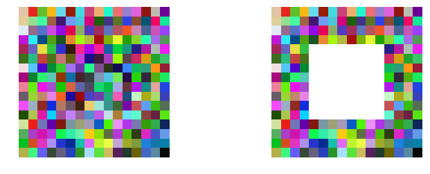
In the example below we will create a 16x16 pixel, 3 channels random icon example.
np.random.seed(42)
torch.manual_seed(42)
# PyTorch channel-first convention
random_icon = torch.rand(3,16,16)
tensor_properties(random_icon, show_value=False)
Tensor properties:
rank        : 3
shape       : torch.Size([3, 16, 16])
data type   : torch.float32
tensor type : torch.FloatTensor
Let us plot the random icon using matplotlib. However, before we do so we need to make the format channel-last since that is what matplotlib expects. This can be easily achieved using the torch.Tensor.permute function. We will then modify the data in cl_random_icon to insert an 8x8 pixels white square centred in the icon and plot that as well. To modify cl_radnom_icon we are using what is called indexing. We will introduce slicing and indexing shortly. You might want to revisit the following code then to learn how it works exactly.
cl_random_icon = random_icon.permute(1,2,0)
fig, axes = plt.subplots(1,2, figsize=(12, 4))
axes[0].axis("off")
axes[0].imshow(cl_random_icon.numpy())
cl_random_icon[4:12,4:12] = 1
axes[1].imshow(cl_random_icon.numpy())
axes[1].axis("off")
plt.show()
Selecting Tensor Type
Here we are initializing a tensor with integer values but want to create a float tensor.
cast_float_vector = torch.FloatTensor([7,19,3,4])
tensor_properties(cast_float_vector)
Tensor properties:
rank        : 1
shape       : torch.Size([4])
data type   : torch.float32
tensor type : torch.FloatTensor
value       : tensor([ 7., 19.,  3.,  4.])
Casting Tensor Type
In this example, we are going to cast an existent integer (long) tensor to float.
tensor_properties(vector)
vector = vector.type(torch.FloatTensor)
tensor_properties(vector)
Tensor properties:
rank        : 1
shape       : torch.Size([4])
data type   : torch.int64
tensor type : torch.LongTensor
value       : tensor([ 7, 19,  3,  4])
Tensor properties:
rank        : 1
shape       : torch.Size([4])
data type   : torch.float32
tensor type : torch.FloatTensor
value       : tensor([ 7., 19.,  3.,  4.])
Tensor from NumPy Array and Back
numpy_array = np.array([2,4,6,8,10])
print('Original NumPy array: {0}\n'.format(numpy_array))

even_tensor = torch.from_numpy(numpy_array)
tensor_properties(even_tensor)

back_to_numpy = even_tensor.numpy()
print('\nNumPy array from tensor: {0}'.format(back_to_numpy))
Original NumPy array: [ 2  4  6  8 10]

Tensor properties:
rank        : 1
shape       : torch.Size([5])
data type   : torch.int64
tensor type : torch.LongTensor
value       : tensor([ 2,  4,  6,  8, 10])

NumPy array from tensor: [ 2  4  6  8 10]
Tensor from Pandas Series and Back
pandas_series = pd.Series([2,3,5,7,11,13,17,19])
print('Original Pandas series: {0}\n'.format(pandas_series))
tensor_from_series = torch.from_numpy(pandas_series.values)
tensor_properties(tensor_from_series)
back_to_pandas = pd.Series(tensor_from_series.numpy())
print('\nPandas series from tensor: {0}'.format(back_to_pandas))
Original Pandas series: 0     2
1     3
2     5
3     7
4    11
5    13
6    17
7    19
dtype: int64

Tensor properties:
rank        : 1
shape       : torch.Size([8])
data type   : torch.int64
tensor type : torch.LongTensor
value       : tensor([ 2,  3,  5,  7, 11, 13, 17, 19])

Pandas series from tensor: 0     2
1     3
2     5
3     7
4    11
5    13
6    17
7    19
dtype: int64
Basic Indexing and Slicing of Tensors
We start by creating a 1D tensor with five random numbers.
np.random.seed(42)
t = torch.FloatTensor(np.random.rand(5))
tensor_properties(t)
Tensor properties:
rank        : 1
shape       : torch.Size([5])
data type   : torch.float32
tensor type : torch.FloatTensor
value       : tensor([0.3745, 0.9507, 0.7320, 0.5987, 0.1560])
Next, we want to change the second element, present at index 1 since tensors have a zero-based index, to 1.
t[1] = 1.0
t
tensor([0.3745, 1.0000, 0.7320, 0.5987, 0.1560])
To change multiple elements, we can specify a range of indices. In the example below, we change the third and fourth elements to zero.
t[2:4] = 0
t
tensor([0.3745, 1.0000, 0.0000, 0.0000, 0.1560])
Indexing in PyTorch tensors works just like in Python lists. One final example will illustrate slicing, to assign a range of values from one tensor to another. In this instance, we are going to assign the sixth, seventh and eigth values from tensor s to the second, third and fourth values in tensor t.
s = torch.FloatTensor(np.random.rand(10))
print('t = {0}'.format(t))
print('s = {0}'.format(s))
t[1:4] = s[5:8]
print('t = {0}'.format(t))
t = tensor([0.3745, 1.0000, 0.0000, 0.0000, 0.1560])
s = tensor([0.1560, 0.0581, 0.8662, 0.6011, 0.7081, 0.0206, 0.9699, 0.8324, 0.2123,
        0.1818])
t = tensor([0.3745, 0.0206, 0.9699, 0.8324, 0.1560])
Basic Operations On Tensors
Adding and Subtracting Tensors
Tensors in PyTorch can be easily added or subtracted, using as expected the + and - operators respectively.
u = torch.tensor([1,2])
v = torch.tensor([3,4])
print('u+v = {0}'.format(u+v))
print('u-v = {0}'.format(u-v))
u+v = tensor([4, 6])
u-v = tensor([-2, -2])
Adding a 3D tensor to a 2D tensor is also straightforward. PyTorch uses broadcasting to repeat the addition of the 2D tensor to each 2D tensor element present in the 3D tensor. It does this without actually making copies of the data. Also certain properties must be satisfied, for instance some dimensions must match, for PyTorch to be able to broadcast. You can read more about the specific details here.
u = torch.tensor([[[1,2],[3,4]],[[0,1],[1,0]]])
v = torch.tensor([[4,5],[6,7]])
print('u+v = {0}'.format(u+v))
print('u-v = {0}'.format(u-v))
u+v = tensor([[[ 5,  7],
         [ 9, 11]],

        [[ 4,  6],
         [ 7,  7]]])
u-v = tensor([[[-3, -3],
         [-3, -3]],

        [[-4, -4],
         [-5, -7]]])
Adding a Constant to a Tensor
u = torch.tensor([[[1,2],[3,4]],[[0,1],[1,0]]])
print('u+3 = {0}'.format(u+3))
u+3 = tensor([[[4, 5],
         [6, 7]],

        [[3, 4],
         [4, 3]]])
Multiplying Tensors With Scalars
u = torch.tensor([[[1,2],[3,4]],[[0,1],[1,0]]])
v = torch.tensor([[4,5],[6,7]])
print('u*3 = {0}'.format(u*3))
print('v*2 = {0}'.format(v*2))
u*3 = tensor([[[ 3,  6],
         [ 9, 12]],

        [[ 0,  3],
         [ 3,  0]]])
v*2 = tensor([[ 8, 10],
        [12, 14]])
Product of Two Tensors
The product of two tensors $u \circ v$ is computed using the hadamard product.
u = torch.tensor([[1,2],[3,4]])
v = torch.tensor([[4,5],[6,7]])
print('u*v = {0}'.format(u*v))
u*v = tensor([[ 4, 10],
        [18, 28]])
Dot Product
The dot product of two 1D tensors, i.e. vectors, say $u$ and $v$, is computed as $u^Tv$. This can computed in PyTorch using the torch.dot function.
u = torch.tensor([1,2,3,4])
v = torch.tensor([4,5,6,7])
print('uv = {0}'.format(torch.dot(u,v)))
uv = 60
Mean, Standard Deviation, Min, Median and Max of Tensor
u = torch.FloatTensor([[[1,2],[3,4]],[[0,1],[1,0]]])
print('mean of u = {0}'.format(u.mean()))

print('std of u = {0}'.format(u.std()))
print('min of u = {0}'.format(u.min()))
print('median of u = {0}'.format(u.median()))
print('max of u = {0}'.format(u.max()))
mean of u = 1.5
std of u = 1.4142135381698608
min of u = 0.0
median of u = 1.0
max of u = 4.0
Multiplying Two 2D Tensors (Matrices)
# 2x3 matrix
N = torch.tensor([[1,2,3],[4,5,6]])
# 3x2 matrix
M = torch.tensor([[1,2],[3,4],[5,6]])
NM = torch.mm(N,M)
print('NM = [2x3] x [3x2] = [2x2]')
print(NM)
print(NM.shape)
NM = [2x3] x [3x2] = [2x2]
tensor([[22, 28],
        [49, 64]])
torch.Size([2, 2])
Computing Gradients
The backpropagation method is used by gradient descent optimization algorithms to adjust the weights of neural networks. This is done by computing the gradient of the loss function and then adjusting weights along the neural network using the chain rule. If you need to learn how backpropagation works, work through chapter 2, How the backpropagation algorithm works, of Michael Nielsen’s Neural Networks and Deep Learning free online book.
Let us go through a couple of examples of differentiation and partial derivatives to jog our memory.
Suppose we have a function $f(x) = 3x^2$. The derivative with respect to $x$ is $f^\prime(x) = \frac{\delta f(x)}{\delta x} = 6x$.
Now suppose we have a function $h(x,y) = 2x^2 + xy$. The partial derivatives with respect to each variable are $\frac{\partial h(x,y)}{\partial x} = 4x + y$ and $\frac{\partial h(x,y)}{\partial y} = x$. The gradient of a function, denoted $\nabla f$, is a vector whose elements are the partial derivatives of the function with respect to each independent variable.
In our example, $\nabla h(x,y) = \left( \frac{\partial h(x,y)}{\partial x}, \frac{\partial h(x,y)}{\partial y} \right)$.
Having determined the derivate function for both example functions $f(x)$ and $h(x,y)$, we can now compute the derivate and gradient respectively at any given point.
For $f(x)$, the derivative at $x=2$ is $f^\prime(2)=\frac{\delta f}{\delta x}= 6x = 6 \times 2 = 12$.
For $h(x,y)$, the gradient at $x=2$ and $y=2$ is $\nabla h(x,y) = \left( \frac{\partial h(x,y)}{\partial x}, \frac{\partial h(x,y)}{\partial y} \right) = \left( 4x + y, x \right) = \left( 4 \times 2 + 2, 2 \right) = \left( 10, 2 \right)$.
Let us now see how this can be done in PyTorch, first for $f(x) = 3x^2$.
x = torch.tensor(2., requires_grad=True)

f = 3*x**2
f.backward()
print('Derivative at x=2: {0}'.format(x.grad))
Derivative at x=2: 12.0
Next, we compute the gradient for $h(x,y) = 2x^2 + xy$ when $x=2$ and $y=2$.
x = torch.tensor(2., requires_grad=True)
y = torch.tensor(2., requires_grad=True)

h = 2*x**2 + x*y
h.backward()
print('Gradient at x=2 and y=2: ({0}, {1})'.format(x.grad, y.grad))
Gradient at x=2 and y=2: (10.0, 2.0)
Conclusion
In this notebook, we have learnt what tensors are and what they are typically used for in machine learning applications. We then explored the most common types of tensors, from 0D to 5D and how to create them in PyTorch. Furthermore, we explored how we can cast PyTorch tensors back and forth from NumPy and Pandas arrays and series respectively and how to index and slice tensors. We also went through some common operations on tensors, such as addition, scaling, dot products and matrix multiplication. Finally, we quickly revised what differentiation and partial differentiation is and how it can be computed using PyTorch.