
CIFAR-10 Classifier Using CNN in PyTorch
In this notebook we will use PyTorch to construct a convolutional neural network. We will then train the CNN on the CIFAR-10 data set to be able to classify images from the CIFAR-10 testing set into the ten categories present in the data set.
CIFAR-10
The CIFAR-10 data set is composed of 60,000 32x32 colour images, 6,000 images per class, so 10 categories in total. The training set is made up of 50,000 images, while the remaining 10,000 make up the testing set.
The categories are: airplane, automobile, bird, cat, deer, dog, frog, horse, ship and truck.
More information regarding the CIFAR-10 and CIFAR-100 data sets can be found here.
Importing Libraries
import torch
import torchvision
import torchvision.transforms as transforms
Downloading, Loading and Normalising CIFAR-10
PyTorch provides data loaders for common data sets used in vision applications, such as MNIST, CIFAR-10 and ImageNet through the torchvision package. Other handy tools are the torch.utils.data.DataLoader that we will use to load the data set for training and testing and the torchvision.transforms, which we will use to compose a two-step process to prepare the data for use with the CNN.
# This is the two-step process used to prepare the
# data for use with the convolutional neural network.

# First step is to convert Python Image Library (PIL) format
# to PyTorch tensors.

# Second step is used to normalize the data by specifying a
# mean and standard deviation for each of the three channels.
# This will convert the data from [0,1] to [-1,1]

# Normalization of data should help speed up conversion and
# reduce the chance of vanishing gradients with certain
# activation functions.
transform = transforms.Compose(
    [transforms.ToTensor(),
     transforms.Normalize((0.5, 0.5, 0.5), (0.5, 0.5, 0.5))])

trainset = torchvision.datasets.CIFAR10(root='./data/',
                                        train=True,
                                        download=True,
                                        transform=transform)
trainloader = torch.utils.data.DataLoader(trainset,
                                          batch_size=4,
                                          shuffle=True)

testset = torchvision.datasets.CIFAR10(root='./data',
                                       train=False,
                                       download=True,
                                       transform=transform)
testloader = torch.utils.data.DataLoader(testset,
                                         batch_size=4,
                                         shuffle=False)

classes = ('plane', 'car', 'bird', 'cat', 'deer',
           'dog', 'frog', 'horse', 'ship', 'truck')
Files already downloaded and verified
Files already downloaded and verified
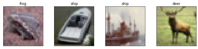
Display Random Batch of 4 Training Images
Using the trainloader we will now get a random batch of 4 training images and plot them to see what CIFAR-10 images look like.
import matplotlib.pyplot as plt
import numpy as np

def convert_to_imshow_format(image):
    # first convert back to [0,1] range from [-1,1] range
    image = image / 2 + 0.5
    image = image.numpy()
    # convert from CHW to HWC
    # from 3x32x32 to 32x32x3
    return image.transpose(1,2,0)

dataiter = iter(trainloader)
images, labels = dataiter.next()

fig, axes = plt.subplots(1, len(images), figsize=(12,2.5))
for idx, image in enumerate(images):
    axes[idx].imshow(convert_to_imshow_format(image))
    axes[idx].set_title(classes[labels[idx]])
    axes[idx].set_xticks([])
    axes[idx].set_yticks([])
Defining the Convolutional Neural Network
The network has the following layout,
Input > Conv (ReLU) > MaxPool > Conv (ReLU) > MaxPool > FC (ReLU) > FC (ReLU) > FC (SoftMax) > 10 outputs
where:
Conv is a convolutional layer, ReLU is the activation function, MaxPool is a pooling layer, FC is a fully connected layer and SoftMax is the activation function of the output layer.
Layer Dimensions
Input Size
The images are 3x32x32, i.e., 3 channels (red, green, blue) each of size 32x32 pixels.
First Convolutional Layer
The first convolutional layer expects 3 input channels and will convolve 6 filters each of size 3x5x5. Since padding is set to 0 and stride is set to 1, the output size is 6x28x28, because $\left( 32-5 \right) + 1 = 28$. This layer therefore has $\left( \left( 5 \times 5 \times 3 \right) + 1 \right) \times 6 = 456$ parameters.
First Max-Pooling Layer
The first down-sampling layer uses max pooling with a 2x2 kernel and stride set to 2. This effectively drops the size from 6x28x28 to 6x14x14.
Second Convolutional Layer
The second convolutional layers expects 6 input channels and will convolve 16 filters each of size 6x5x5. Since padding is set to 0 and stride is set to 1, the output size is 16x10x10, because $\left( 14-5 \right) + 1 = 10$. This layer therefore has $\left( \left( 5 \times 5 \times 6 \right) + 1 \right) \times 16 = 2416$ parameters.
Second Max-Pooling Layer
The second down-sampling layer uses max pooling with a 2x2 kernel and stride set to 2. This effectively drops the size from 16x10x10 to 16x5x5.
First Fully-Connected Layer
The output from the final max pooling layer needs to be flattened so that we can connect it to a fully connected layer. This is achieved using the torch.Tensor.view method. By specifying -1 the method will automatically infer the number of rows required. This is done to handle the mini-batch size of data.
The fully-connected layer uses ReLU for activation and has 120 nodes, thus in total it needs $\left( \left( 16 \times 5 \times 5 \right) + 1 \right) \times 120 = 48120$ parameters.
Second Fully-Connected Layer
The output from the first fully-connected layer is connected to another fully connected layer with 84 nodes, using ReLU as an activation function. This layer thus needs $\left( 120 + 1 \right) \times 84 = 10164$ parameters.
Output Layer
The last fully-connected layer uses softmax and is made up of ten nodes, one for each category in CIFAR-10. This layer requires $\left( 84 + 1 \right) \times 10 = 850$ parameters.
Total Network Parameters
This convolutional neural network has a total of $456 + 2416 + 48120 + 10164 + 850 = 62006$ parameters.
import torch.nn as nn
import torch.nn.functional as F

class Net(nn.Module):
    def __init__(self):
        super(Net, self).__init__()
        self.conv1 = nn.Conv2d(3, 6, 5)
        self.pool = nn.MaxPool2d(2, 2)
        self.conv2 = nn.Conv2d(6, 16, 5)
        self.fc1 = nn.Linear(16 * 5 * 5, 120)
        self.fc2 = nn.Linear(120, 84)
        self.fc3 = nn.Linear(84, 10)

    def forward(self, x):
        x = self.pool(F.relu(self.conv1(x)))
        x = self.pool(F.relu(self.conv2(x)))
        x = x.view(-1, 16 * 5 * 5)
        x = F.relu(self.fc1(x))
        x = F.relu(self.fc2(x))
        x = self.fc3(x)
        return x

net = Net()
Defining the Loss Function and Optimizer
Since we are classifying images into more than two classes we will use cross-entropy as a loss function. To optimize the network we will employ stochastic gradient descent (SGD) with momentum to help get us over local minima and saddle points in the loss function space.
import torch.optim as optim

criterion = nn.CrossEntropyLoss()
optimizer = optim.SGD(net.parameters(), lr=0.001, momentum=0.9)
Training the Network
We will now train the network using the trainloader data, by going over all the training data in batches of 4 images, and repeating the whole process 2 times, i.e., 2 epochs. Every 2000 batches we report on training progress by printing the current epoch and batch number along with the running loss value.
Once training is complete, we will save the model parameters to disk. This will make it possible to load the model parameters from disk the next time we run this notebook and thus not have to train the model again, saving some time. More details on how to save and load model parameters can be found here.
import os

epochs = 2

model_directory_path = 'model/'
model_path = model_directory_path + 'cifar-10-cnn-model.pt'

if not os.path.exists(model_directory_path):
    os.makedirs(model_directory_path)

if os.path.isfile(model_path):
    # load trained model parameters from disk
    net.load_state_dict(torch.load(model_path))
    print('Loaded model parameters from disk.')
else:
    for epoch in range(epochs):  # loop over the dataset multiple times

        running_loss = 0.0
        for i, data in enumerate(trainloader, 0):
            # get the inputs
            inputs, labels = data

            # zero the parameter gradients
            optimizer.zero_grad()

            # forward + backward + optimize
            outputs = net(inputs)
            loss = criterion(outputs, labels)
            loss.backward()
            optimizer.step()

            # print statistics
            running_loss += loss.item()
            if i % 2000 == 1999:    # print every 2000 mini-batches
                print('[%d, %5d] loss: %.3f' %
                      (epoch + 1, i + 1, running_loss / 2000))
                running_loss = 0.0
    print('Finished Training.')
    torch.save(net.state_dict(), model_path)
    print('Saved model parameters to disk.')
Loaded model parameters from disk.
Testing the Network
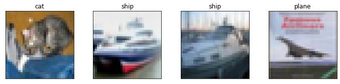
Now that the network is trained we can evaluate how it performs on the testing data set. Let us load four random images from the testing data set and their corresponding labels.
dataiter = iter(testloader)
images, labels = dataiter.next()

fig, axes = plt.subplots(1, len(images), figsize=(12,2.5))
for idx, image in enumerate(images):
    axes[idx].imshow(convert_to_imshow_format(image))
    axes[idx].set_title(classes[labels[idx]])
    axes[idx].set_xticks([])
    axes[idx].set_yticks([])
Next, we input the four images to the trained network to get class (label/category) predictions.
outputs = net(images)
The network outputs a 2D tensor (array) of size 4x10, a row for each image and a column for each category. The values are raw outputs from the linear transformation $y = xA^T + b$. The category predicted for each image (row) is thus the column index containing the maximum value in that row.
outputs
tensor([[ 0.3214, -0.1016,  0.4087,  1.6078, -1.3790,  0.2655, -0.7055, -0.6274,
          0.4320, -0.0205],
        [ 5.4812,  7.9856, -1.7315, -1.3632, -5.0847, -3.8232, -5.6879, -4.3160,
          6.2993,  3.8083],
        [ 3.0471,  3.5417, -0.1734, -0.6367, -1.8952, -2.1822, -2.8114, -1.9013,
          2.7827,  1.6128],
        [ 3.8433,  2.4575,  0.5930, -0.3768, -2.1527, -2.2164, -2.9778, -2.9104,
          3.6113,  1.2065]], grad_fn=<AddmmBackward>)
If we prefer to get a probability score, we can use the nn.Softmax function on the raw output as follows.
sm = nn.Softmax(dim=1)
sm_outputs = sm(outputs)
print(sm_outputs)
tensor([[9.9337e-02, 6.5070e-02, 1.0840e-01, 3.5955e-01, 1.8140e-02, 9.3933e-02,
         3.5575e-02, 3.8461e-02, 1.1096e-01, 7.0573e-02],
        [6.3723e-02, 7.7977e-01, 4.6974e-05, 6.7891e-05, 1.6428e-06, 5.8003e-06,
         8.9876e-07, 3.5438e-06, 1.4442e-01, 1.1962e-02],
        [2.6785e-01, 4.3926e-01, 1.0697e-02, 6.7305e-03, 1.9120e-03, 1.4349e-03,
         7.6483e-04, 1.9004e-03, 2.0563e-01, 6.3824e-02],
        [4.5973e-01, 1.1499e-01, 1.7821e-02, 6.7572e-03, 1.1441e-03, 1.0736e-03,
         5.0136e-04, 5.3631e-04, 3.6454e-01, 3.2912e-02]],
       grad_fn=<SoftmaxBackward>)
Predicted Category for Four Test Images
probs, index = torch.max(sm_outputs, dim=1)

for p, i in zip(probs, index):
    print('{0} - {1:.4f}'.format(classes[i], p))
cat - 0.3596
car - 0.7798
car - 0.4393
plane - 0.4597
The model got half of the four testing images correct. It correctly categorised the cat and plane images, but failed on the two ship images, instead categorising them as cars. Let us now evaluate the model on the whole testing set.
Predicting the Category for all Test Images
total_correct = 0
total_images = 0
confusion_matrix = np.zeros([10,10], int)
with torch.no_grad():
    for data in testloader:
        images, labels = data
        outputs = net(images)
        _, predicted = torch.max(outputs.data, 1)
        total_images += labels.size(0)
        total_correct += (predicted == labels).sum().item()
        for i, l in enumerate(labels):
            confusion_matrix[l.item(), predicted[i].item()] += 1

model_accuracy = total_correct / total_images * 100
print('Model accuracy on {0} test images: {1:.2f}%'.format(total_images, model_accuracy))
Model accuracy on 10000 test images: 52.20%
The model performed much better than random guessing, which would give us an accuracy of 10% since there are ten categories in CIFAR-10. Let us now use the confusion matrix to compute the accuracy of the model per category.
print('{0:10s} - {1}'.format('Category','Accuracy'))
for i, r in enumerate(confusion_matrix):
    print('{0:10s} - {1:.1f}'.format(classes[i], r[i]/np.sum(r)*100))
Category   - Accuracy
plane      - 53.5
car        - 82.7
bird       - 61.0
cat        - 25.4
deer       - 32.9
dog        - 40.2
frog       - 43.7
horse      - 63.7
ship       - 73.8
truck      - 45.1
Finally, let us visualise the confusion matrix to determine common misclassifications.
fig, ax = plt.subplots(1,1,figsize=(8,6))
ax.matshow(confusion_matrix, aspect='auto', vmin=0, vmax=1000, cmap=plt.get_cmap('Blues'))
plt.ylabel('Actual Category')
plt.yticks(range(10), classes)
plt.xlabel('Predicted Category')
plt.xticks(range(10), classes)
plt.show()
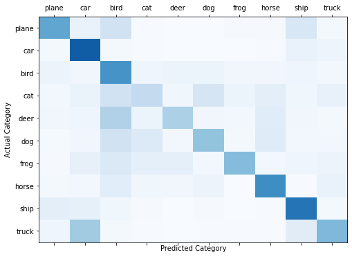
From the above visualisation we can see that the best accuracy was achieved on the car and ship categories, darkest shades present on the main diagonal. The truck category was most frequently confused with the car category. This is understandable, since they are both vehicles and have some visual similarities. Planes were also commonly confused with bird and ship. This could have something to do with a common background texture and colour, blue for both sky and sea.
To understand precisely which categories were most commonly confused, we can print the absolute and relative values of the confusion matrix, as follows.
print('actual/pred'.ljust(16), end='')
for i,c in enumerate(classes):
    print(c.ljust(10), end='')
print()
for i,r in enumerate(confusion_matrix):
    print(classes[i].ljust(16), end='')
    for idx, p in enumerate(r):
        print(str(p).ljust(10), end='')
    print()

    r = r/np.sum(r)
    print(''.ljust(16), end='')
    for idx, p in enumerate(r):
        print(str(p).ljust(10), end='')
    print()
actual/pred     plane     car       bird      cat       deer      dog       frog      horse     ship      truck
plane           535       68        195       4         3         2         10        8         153       22
                0.535     0.068     0.195     0.004     0.003     0.002     0.01      0.008     0.153     0.022
car             22        827       16        7         2         2         3         4         68        49
                0.022     0.827     0.016     0.007     0.002     0.002     0.003     0.004     0.068     0.049
bird            55        35        610       40        60        59        35        35        42        29
                0.055     0.035     0.61      0.04      0.06      0.059     0.035     0.035     0.042     0.029
cat             26        64        189       254       38        168       52        95        38        76
                0.026     0.064     0.189     0.254     0.038     0.168     0.052     0.095     0.038     0.076
deer            33        40        319       54        329       33        24        117       32        19
                0.033     0.04      0.319     0.054     0.329     0.033     0.024     0.117     0.032     0.019
dog             14        33        193       136       27        402       22        121       24        28
                0.014     0.033     0.193     0.136     0.027     0.402     0.022     0.121     0.024     0.028
frog            8         81        140       86        93        30        437       29        41        55
                0.008     0.081     0.14      0.086     0.093     0.03      0.437     0.029     0.041     0.055
horse           23        24        108       39        35        56        3         637       7         68
                0.023     0.024     0.108     0.039     0.035     0.056     0.003     0.637     0.007     0.068
ship            98        84        38        9         1         8         1         6         738       17
                0.098     0.084     0.038     0.009     0.001     0.008     0.001     0.006     0.738     0.017
truck           41        361       16        4         1         5         5         6         110       451
                0.041     0.361     0.016     0.004     0.001     0.005     0.005     0.006     0.11      0.451
Conclusion
In this notebook, we trained a simple convolutional neural network using PyTorch on the CIFAR-10 data set. 50,000 images were used for training and 10,000 images were used to evaluate the performance. The model performed well, achieving an accuracy of 52.2% compared to a baseline of 10%, since there are 10 categories in CIFAR-10, if the model guessed randomly.
To improve the performance we can try adding convolution layers, more filters or more fully connected layers. We could also train the model for more than two epochs while introducing some form of regularisation, such as dropout or batch normalization, so as not to overfit the training data.
Keep in mind that complex models with hundreds of thousands of parameters are computationally more expensive to train and thus you should consider training such models on a GPU enabled machine to speed up the process.