MNIST Using Keras

In this notebook, we will build a simple two-layer feed-forward neural network model using Keras, running on top of TensorFlow. We then train the sequential model using 60,000 MNIST digits and evaluate it on 10,000 MNIST digits.

I put this notebook together to briefly comment the code from chapter 2 of François Chollet’s excellent book, Deep Learning with Python.

Loading the Required Libraries

import matplotlib.pyplot as plt
import numpy as np
from keras.datasets import mnist
from keras import models, layers
from keras.utils import to_categorical

np.random.seed(22)

Using TensorFlow backend.

Loading the MNIST Data Set

Each digit is a monochrome 28 by 28 pixels image. The training set consists of 60,000 images and the testing set of 10,000 images. Each image in the training and testing set has a corresponding label provided, indicating the true value of the digit in the image.

(train_images, train_labels), (test_images, test_labels) = mnist.load_data()

Training and Testing Data Shape and Type

print(train_images.shape)
print(len(train_labels))
print("First 10 labels: {0} -> {1}".format(train_labels[:10], type(train_labels[0])))

(60000, 28, 28)
60000
First 10 labels: [5 0 4 1 9 2 1 3 1 4] -> <class 'numpy.uint8'>

print(test_images.shape)
print(len(test_labels))
print("First 10 labels: {0} -> {1}".format(test_labels[:10], type(test_labels[0])))

(10000, 28, 28)
10000
First 10 labels: [7 2 1 0 4 1 4 9 5 9] -> <class 'numpy.uint8'>

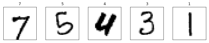
Displaying Random Samples from Training Digits

num_plot_digits = 5
digits_to_plot = np.random.randint(0, 60000, num_plot_digits)
fig, axes = plt.subplots(1, 5, figsize=(12,2))

for i in range(num_plot_digits):
    axes[i].imshow(train_images[digits_to_plot[i]], cmap=plt.cm.binary)
    axes[i].set_title(train_labels[digits_to_plot[i]])
    axes[i].set_xticks([])
    axes[i].set_yticks([])

Network Architecture

Two fully connected (dense) layers, with the first layer using ReLU for activation and the second (last/output) layer using softmax.

network = models.Sequential()
network.add(layers.Dense(512, activation='relu', input_shape=(28 * 28, )))
network.add(layers.Dense(10, activation='softmax'))
network.compile(optimizer='rmsprop',
                loss='categorical_crossentropy',
                metrics=['accuracy'])

Preprocessing Data

The data will be reshaped so that each sample image is a row 784 columns long (28 * 28), as expected by the network. Furthermore, the data will be normalized so all values are in the [0,1] interval and their type changed to float32 from uint8.

The labels will in turn be converted to a categorical type, i.e. one-hot encoded.

train_images = train_images.reshape((60000, 28 * 28))
train_images = train_images.astype('float32') / 255

test_images = test_images.reshape((10000, 28 * 28))
test_images = test_images.astype('float32') / 255

train_labels = to_categorical(train_labels)
test_labels = to_categorical(test_labels)

Training the Network

Fitting the model to the training data using 5 epochs and a batch size of 128.

network.fit(train_images, train_labels, epochs=5, batch_size=128)

Epoch 1/5
60000/60000 [==============================] - 15s 254us/step - loss: 0.2599 - acc: 0.9238
Epoch 2/5
60000/60000 [==============================] - 15s 257us/step - loss: 0.1045 - acc: 0.9691
Epoch 3/5
60000/60000 [==============================] - 15s 258us/step - loss: 0.0695 - acc: 0.9790
Epoch 4/5
60000/60000 [==============================] - 16s 263us/step - loss: 0.0501 - acc: 0.9847
Epoch 5/5
60000/60000 [==============================] - 16s 264us/step - loss: 0.0379 - acc: 0.9886





<keras.callbacks.History at 0x7fe2d3a750b8>

Testing the Network

Testing the accuracy of the fitted model on the testing data set.

test_loss, test_acc = network.evaluate(test_images, test_labels)
print('loss: {0:.4f} - acc: {1:.4f}'.format(test_loss, test_acc))

10000/10000 [==============================] - 2s 192us/step
loss: 0.0651 - acc: 0.9806

Conclusion

This simple two-layer dense sequential network manages an accuracy of 98.86% on the training data set and 98.06% on the testing data set. Much better results can be achieved, well above 99% accuracy, using various ways. For instance, convolutional neural networks. Refer to Yann LeCun’s MNIST page for details of other approaches and the test error rate achieved.