
Concrete Compressive Strength Regression Model Using Keras
In this notebook, we will build a simple three-layer feed-forward neural network model using Keras, running on top of TensorFlow. The sequential model will be trained using the Concrete Compressive Strength Data Set to learn to predict the compressive strength of concrete samples based on the material used to make them.
Loading the Required Libraries
import pandas as pd
from pathlib import Path
from sklearn import model_selection
from sklearn import preprocessing
import matplotlib.pyplot as plt
from keras import models, layers, metrics

# ensure same network weights at initialisation between notebook runs
import numpy as np
np.random.seed(22)
Using TensorFlow backend.
Loading the Concrete Data Set
concrete_data_file = Path('concrete_data.csv')
if concrete_data_file.is_file():
    print('Reading concrete_data.csv...')
    concrete_data = pd.read_csv('concrete_data.csv')
    print('Done.')
else:
    print('Downloading concrete data CSV file...')
    # Original Source: http://archive.ics.uci.edu/ml/datasets/concrete+compressive+strength
    root_path = 'https://www.stefanfiott.com/machine-learning/'
    folder = 'concrete-compressive-strength-regression-model-using-keras/'
    concrete_data = pd.read_csv(root_path + folder + 'concrete_data.csv')
    print('Done.')
    print('Saving to concrete_data.csv file...')
    concrete_data.to_csv('concrete_data.csv', index=False)
    print('Done.')

print(concrete_data.head())
Reading concrete_data.csv...
Done.
   Cement  Blast Furnace Slag  Fly Ash  Water  Superplasticizer  \
0   540.0                 0.0      0.0  162.0               2.5
1   540.0                 0.0      0.0  162.0               2.5
2   332.5               142.5      0.0  228.0               0.0
3   332.5               142.5      0.0  228.0               0.0
4   198.6               132.4      0.0  192.0               0.0

   Coarse Aggregate  Fine Aggregate  Age  Strength
0            1040.0           676.0   28     79.99
1            1055.0           676.0   28     61.89
2             932.0           594.0  270     40.27
3             932.0           594.0  365     41.05
4             978.4           825.5  360     44.30
Preparing the Training and Testing Data Sets
We will now separate the data into independent (predictor) variables and dependent (outcome) variables.
predictors = concrete_data.iloc[:,0:8].values
outcomes = concrete_data.iloc[:,8].values
Next, we scale the predictor variables to reduce variance, so all values are in the [0,1] interval. This should help the model train faster and better.
min_max_scaler = preprocessing.MinMaxScaler()
predictors_scaled = min_max_scaler.fit_transform(predictors)
predictors_scaled[:5,]
array([[1.        , 0.        , 0.        , 0.32108626, 0.07763975,
        0.69476744, 0.20572002, 0.07417582],
       [1.        , 0.        , 0.        , 0.32108626, 0.07763975,
        0.73837209, 0.20572002, 0.07417582],
       [0.52625571, 0.39649416, 0.        , 0.84824281, 0.        ,
        0.38081395, 0.        , 0.73901099],
       [0.52625571, 0.39649416, 0.        , 0.84824281, 0.        ,
        0.38081395, 0.        , 1.        ],
       [0.22054795, 0.36839176, 0.        , 0.56070288, 0.        ,
        0.51569767, 0.58078274, 0.98626374]])
Finally, we split the data into a training set and a testing set. These will in turn be used to train and evaluate the regression model respectively.
X_train, X_test, y_train, y_test = model_selection.train_test_split(predictors, outcomes, test_size=0.33, random_state=22)
print('X_train {0}, y_train {1}'.format(X_train.shape, y_train.shape))
print('X_test {0}, y_test {1}'.format(X_test.shape, y_test.shape))
X_train (690, 8), y_train (690,)
X_test (340, 8), y_test (340,)
Network Architecture
Three fully connected (dense) layers, with the first and second layer using ReLU for activation and the third (last/output) layer is a linear combination of its inputs.
network = models.Sequential()
network.add(layers.Dense(10, activation='relu', input_shape=(X_train.shape[1], )))
network.add(layers.Dense(5, activation='relu'))
network.add(layers.Dense(1))
network.compile(optimizer='adam',
                loss='mean_squared_error')
Training and Testing the Network
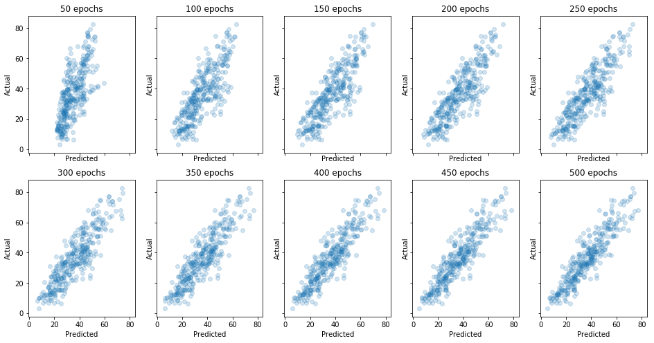
We will now fit the model to the training data using 50 epochs and a batch size of 128. Then we evaluate the performance of the trained network against the testing data. We will draw a scatter plot of predicted values against actual values. The better the predictions the tighter together the plot will be and in a perfect model the points would line-up along the minor diagonal, i.e., a line from bottom left to top right. To observe how the model starts fitting the data better with more training, we will repeat this process 10 times, each time plotting a new predictions scatter plot.
By the end of the training the model will have gone through 500 epochs.
fig, axes = plt.subplots(2, 5, figsize=(16,8), sharex=True, sharey=True)
losses = []
for i in range(2):
    for j in range(5):
        network.fit(X_train, y_train, epochs=50, batch_size=128, verbose=0);
        pred_loss = network.evaluate(X_test, y_test, verbose=0)
        losses.append(pred_loss)
        preds = network.predict(X_test)
        axes[i,j].scatter(preds, y_test, alpha=0.2)
        axes[i,j].set_title('{0} epochs'.format((5*i+j+1)*50))
        axes[i,j].set_ylabel('Actual')
        axes[i,j].set_xlabel('Predicted')
fig, ax = plt.subplots(1, 1, figsize=(10, 5))
ax.plot(losses)
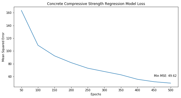
ax.set_title('Concrete Compressive Strength Regression Model Loss')
epochs = [str(i*50) for i in range(1, len(losses)+1)]
ax.set_xticks(range(len(losses)))
ax.set_xticklabels(epochs)
ax.set_xlabel('Epochs')
ax.set_ylabel('Mean Squared Error')
ax.text(len(losses)-2, losses[len(losses)-1]+10, 'Min MSE: {0:.2f}'.format(losses[len(losses)-1]));
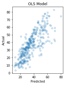
Comparing Performance to Ordinary Least Squares (OLS) Regression Model
We will now model the same training data using an ordinary least squares (OLS) regression model using Scikit-learn and then evaluate it on the same testing data set we used before.
from sklearn import linear_model
from sklearn.metrics import mean_squared_error

regr = linear_model.LinearRegression()
regr.fit(X_train, y_train)
ols_y_pred = regr.predict(X_test)

fig, ax = plt.subplots(1, 1, figsize=(3,4))
ax.scatter(ols_y_pred, y_test, alpha=0.2)
ax.set_title('OLS Model'.format((5*i+j+1)*50))
ax.set_ylabel('Actual')
ax.set_xlabel('Predicted')

print("Mean squared error: {0:.2f}".format(mean_squared_error(y_test, ols_y_pred)))
Mean squared error: 105.37
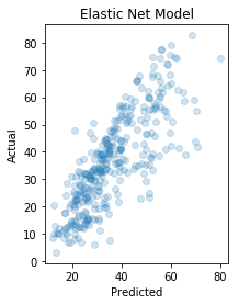
Comparing Performance to Elastic Net Model
We will now model the same training data using an Elastic Net model using Scikit-learn. Elastic net uses both lasso (L1) and ridge regression (L2), resulting in a sparser model while still penalizing large coefficients. Finally, we evaluate it on the same testing data set we used with the other models.
from sklearn.linear_model import ElasticNetCV

regr = ElasticNetCV(cv=5)
regr.fit(X_train, y_train)

elastic_y_pred = regr.predict(X_test)

fig, ax = plt.subplots(1, 1, figsize=(3,4))
ax.scatter(elastic_y_pred, y_test, alpha=0.2)
ax.set_title('Elastic Net Model'.format((5*i+j+1)*50))
ax.set_ylabel('Actual')
ax.set_xlabel('Predicted')

print("Mean squared error: {0:.2f}".format(mean_squared_error(y_test, elastic_y_pred)))
Mean squared error: 105.63
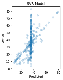
Comparing Performance to Support Vector Regression (SVR) Model
We will now model the same training data using a support vector regression model using Scikit-learn. First, we will tune the model to find optimal hyper-parameters using grid search and cross-validation. Finally, we evaluate the fitted model on the same testing data set we used so far.
from sklearn.svm import SVR
from sklearn.model_selection import GridSearchCV

svr = GridSearchCV(SVR(kernel='rbf', gamma=0.1),
                   cv=5,
                   param_grid={'C': [1e0, 1e1, 1e2, 1e3],
                               'gamma': np.logspace(-2, 2, 5),
                               'epsilon': np.arange(0.1, 0.5, 0.1)})
svr.fit(X_train, y_train)
svr_y_pred = svr.best_estimator_.predict(X_test)
fig, ax = plt.subplots(1, 1, figsize=(3,4))
ax.scatter(svr_y_pred, y_test, alpha=0.2)
ax.set_title('SVR Model'.format((5*i+j+1)*50))
ax.set_ylabel('Actual')
ax.set_xlabel('Predicted')

print("Mean squared error: {0:.2f}".format(mean_squared_error(y_test, svr_y_pred)))
Mean squared error: 190.75
Conclusion
In this notebook we built various models to predict the compressive strength in megapascals (MPa) of concrete depending on the concrete mixture properties. We first created a simple three-layer dense sequential network, achieving a mean-squared error of 49.62. Next, we built an ordinary least squares (OLS) model, an Elastic Net model and finally an SVR model, achieving a mean-squared error of 105.37, 105.63 and 190.75 respectively.
Without any tuning the simple neural network achieves the best mean-squared error. The other models, even after tuning, cannot get below a mean-squared error of 100. Clearly, this is a highly non-linear problem. Therefore, the neural network’s non-linearity and three-layers are better at transforming the data into a representation that can be mapped more accurately to the compressive strength.