Evaluating Binary Classifier Performance

What are Binary Classifiers?

A binary classification model is one that assigns either of two outcomes to the input. This could be a model that detects SPAM, which given a set of features representing an email would output TRUE if it is classified as SPAM email or FALSE otherwise, i.e. HAM email.

Another example would be a medical diagnosis model that based on the input data determines whether a particular disease is present or not.

Possible Outcomes

Since there are two possible actual states, i.e., true/false or positive/negative or 1/0, and the model can predict either one of them, there are in all four possible outcomes as follows.

	Actual True	Actual False
Predicted True	True Positive (TP) Correct Prediction	False Positive (FP) Wrong Prediction
Predicted False	False Negative (FN) Wrong Prediction	True Negative (TN) Correct Prediction

The above table is referred to as a confusion matrix.

Type I Error - False Positive (FP)

A type I error is a false positive, meaning an actual negative was classified as a positive. For example, a HAM email is classified as SPAM, or a legitimate transaction is classified as fraudulent.

In statistical hypothesis testing, a type I error occurs when the null hypothesis $H_0$ is rejected when it is true.

The probability of rejecting the null hypothesis $H_0$ when it is true, the type I error rate or False Positive Rate (FPR), is denoted by $\alpha$ and is called the significance level or alpha level, commonly set to 0.05, which means that it is acceptable to reject $H_0$ when it is true in $5\%$ of the cases.

\[\textit{False Positive Rate (FPR)} = \alpha = \frac{FP}{TN+FP}\]

Type II Error - False Negative (FN)

A type II error is a false negative, meaning an actual positive was classified as a negative. For example, a SPAM email is classified as HAM, or a fraudulent transaction is classified as legitimate.

In statistical hypothesis testing, a type II error occurs when the alternative hypothesis $H_1$ is rejected when it is true.

The probability of rejecting the alternative hypothesis $H_1$ when it is true, the type II error rate or False Negative Rate (FNR), is denoted by $\beta$.

\[\textit{False Negative Rate (FNR)} = \beta = \frac{FN}{TP+FN}\]

Statistical Power

Statistical power is the probability of a binary hypothesis test to reject the null hypothesis $H_0$ when a specific alternative hypothesis $H_1$ is true. In the context of binary classification models, statistical power is called statistical sensitivity or True Positive Rate (TPR).

As statisitical power increases towards $1$, the probability of making a type II error, i.e., a false negative (FP), decreases. In fact, $power=1-\beta$, where $\beta$ is the type II error rate or False Negative Rate (FNR).

\[\textit{True Positive Rate (TPR)} = power = \frac{TP}{TP+FN} = 1 - FNR\]

Accuracy

Accuracy is the ratio of correct predictions to the total number of predictions made.

\[Accuracy=\frac{correct\ predictions}{total\ predictions}=\frac{TP+TN}{TP+TN+FP+FN}\]

For a balanced data set, i.e. one where there is an equal amount of positive and negative outcomes, accuracy is not a bad measure of model performance. Using a balanced data set, if the model always predicted positive, or negative for that matter, the expected accuracy would be $\sim0.5$. Under such a scenario a model that gives high accuracies, say above $0.8$ or $0.9$, will most likely be considered to be performing well.

On the other hand, for an imbalanced data set, for example, a fraud detection system where say, less than $0.1\%$ of transactions are fraudulent, accuracy is not a good measure because a model that always predicts not fraudulent, i.e. negative, will have a very high accuracy of $\sim0.999$.

Precision and Recall

Precision and Recall are two performance measures used in particular in information retrieval tasks. In such context, precision and recall represent the following:

\[Precision=\frac{|\{Relevant\ Documents\} \cap \{Retrieved\ Documents\}|}{|\{Retrieved\ Documents\}|}\] \[Recall=\frac{|\{Relevant\ Documents\} \cap \{Retrieved\ Documents\}|}{|\{Relevant\ Documents\}|}\]

In the context of a binary classifier, precision and recall represent the following:

\[Precision=\frac{TP}{TP+FP}\] \[Recall=\frac{TP}{TP+FN}\]

F-measure

Taking either of precision and recall on their own is not useful. For example, suppose a SPAM detection model is tuned to detect all SPAM emails. In doing so, many HAM emails get classified as SPAM. In this case, the $FN$ will be low or zero, but the $FP$ will be quite high. Therefore, $Recall$ will be close to $1$ while $Precision$ will be low or close to zero.

Therefore, a better measure is the $\textit{F-measure}$ which is the harmonic mean of $Precision$ and $Recall$, computed as follows:

\[\textit{F-measure}=2 \cdot \frac{precision \cdot recall}{precision + recall}\]

Using the $\textit{F-measure}$, if $Recall = 1$ and $Precision = 0$, or vice-versa, then $\textit{F-measure}=0$.

A binary classifier with an $\textit{F-measure}=1$ is a perfect binary classifier, having both perfect precision and recall, i.e., $FP=0$ and $FN=0$ respectively. Therefore, good classifier models have $\textit{F-measure}$ values approaching $1$.

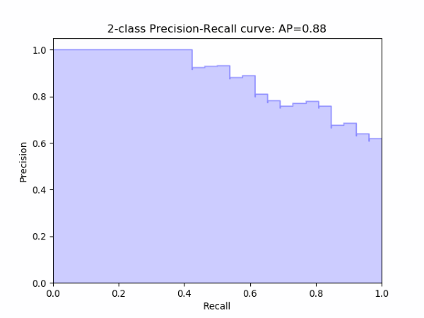
PR-curve

To evaluate a model, the $Precision$ and $Recall$ are computed for various binary classification thresholds and then plotted on a PR-curve, like the one below. Assuming a balanced class data set and equal importance given to both classes, a model with a larger area under the curve, shown below shaded, is better than another model with a smaller area under the curve.

Source: http://scikit-learn.org/stable/auto_examples/model_selection/plot_precision_recall.html

Note: $\textit{F-measure}$, $Precision$, $Recall$ and PR-curves need to be interpreted in the context of the task at hand. For some tasks, say fraud detection, we might want a very low or zero $FN$ rate and can live with some $FP$, if it means detecting all fraudulent activity.

On the other hand, in a SPAM detection system, we might prefer to let some SPAM emails slip by undetected, so have a slightly higher $FN$ rate and a low or zero $FP$ rate, rather than risk blocking a legitimate important email from a potential or existing customer as SPAM.

Sensitivity and Specificity

$Sensitivity$ and $Specificity$ are also known as the True Positive Rate and True Negative Rate respectively and are computed as follows.

\[Sensitivity = \textit{True Positive Rate} = Recall = \frac{TP}{TP+FN}\] \[Specificity = \textit{True Negative Rate} = \frac{TN}{TN+FP} = 1 - FPR\]

$Sensitivity$ and $Specificity$ are used in particular to measure the performance of medical diagnosis models. In the context of testing for the presence of a disease, $Sensitivity$ is a measure of the ability of a medical model to detect a disease if it is present, i.e. high sensitivity would lower $FN$. $Specificity$ is a measure of the ability of a medical model to correctly classify healthy individuals as not having a disease, i.e. high specificity would lower $FP$.

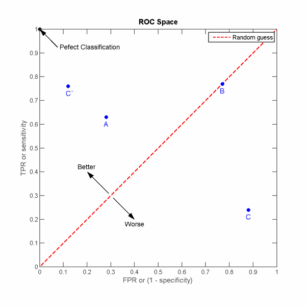
Receiver Operating Characteristic (ROC) curve

The Receiver Operating Characteristic (ROC) curve plots the True Positive Rate (TPR), i.e., Sensitivity or Recall, against the False Positive Rate (FPR), i.e., $1 - Specificity$.

A perfect classifier would thus have high sensitivity, so $FN=0$ and thus $TPR=1$, and a high specificity, so $FP=0$ and thus $1 - TNR = 0$, resulting in the point in the top-left corner on the figure below. Any curve to the left and above of the red dashed line, representing a model classifying randomly, is a better performance than random guessing, and to the right and below is a classifier performing worse than random guessing.

Source: https://en.wikipedia.org/wiki/Receiver_operating_characteristic

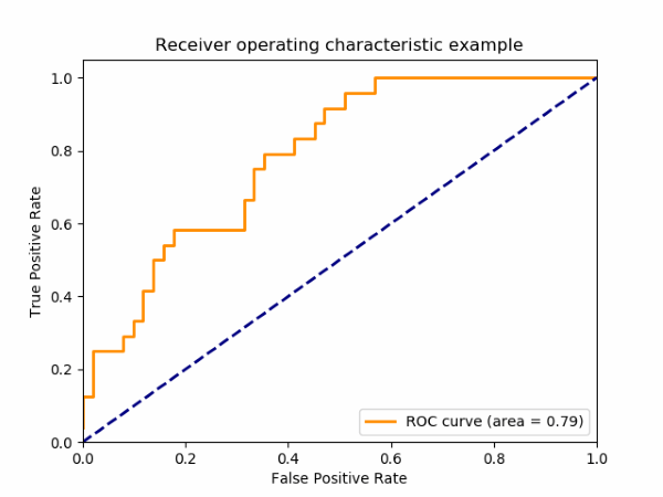
ROC Area Under the Curve (AUC)

The area under the curve (AUC) is an aggregate measure of the performance of a binary classification model across all possible classification thresholds. Remember that a perfect binary classifier would have all points positioned in the top-left corner, representing $TPR=1$ and $FPR=0$ for all classification thresholds. In such a case, the shaded area under the curve would be the whole square and thus $AUC=1$.

Source: http://scikit-learn.org/stable/auto_examples/model_selection/plot_roc.html

In the example ROC plot above, the $AUC=0.79$, which is good. Definitely much better than random guessing. Certain medical diagnosis models aim for an $AUC>0.9$ to be considered useable. However, $AUC$ values like any other measurements should be interpreted within the context of the project goals. For example, for a certain medical condition, doctors might prefer a model with a high or near perfect sensitivity even if it means a lower specificity. In other words, they would much rather flag all patients having a condition along with some people who are healthy rather than miss out on patients with the condition. Keep in mind that medical diagnosis tests are just that, tests, which are meant to help doctors make a differential diagnosis taking into consideration other factors, including other test results and patient symptoms.