Instacart - Model Fitting
In this notebook we will fit simple reordering classifier models using the features extracted from the Instacart Market Basket Analysis dataset provided by Kaggle. Refer to the Instacart Feature Engineering Notebook to explore how the features were extracted.
Note that the models built in this notebook do not fulfill the requirements of the Kaggle competition, i.e. predicting the reordered products in the last order for each customer. However, they can be used to predict whether a product will be reordered or not, and if the output is a probability, a threshold could be used to select the top $n$ reordered products for each customer and predict those for the last order.
Support Functions
from IPython.display import Markdown, display
%matplotlib inline
import matplotlib.pyplot as plt
import pandas as pd
import numpy as np
import scipy.stats
#-------------------------------------------------------------------------
# Functions to load datasets into memory using space efficient data types.

def load_training_data(path):
    training = pd.read_csv(path, dtype={'user_id': np.uint32,
                                        'product_id': np.uint32,
                                        'prod_prob': np.float16,
                                        'aisle_prob': np.float16,
                                        'department_prob': np.float16,
                                        'reorder_prob': np.float16,
                                        'recency_prob': np.float16,
                                        'DTOP_prob': np.float16,
                                        'reordered': np.uint8},
                           usecols=['prod_prob','aisle_prob','department_prob',
                                    'reorder_prob','recency_prob','DTOP_prob',
                                    'reordered'])

    return training

#----------------------------------------------------------------------
# Function to generate markdown output
# Ref: https://stackoverflow.com/a/32035217
def printmd(string):
    display(Markdown(string))
Load Training Data
training_data = load_training_data('training.csv')
training_data.loc[training_data.reordered == 1][:10]
| prod_prob | aisle_prob | department_prob | reorder_prob | recency_prob | DTOP_prob | reordered | |
|---|---|---|---|---|---|---|---|
| 9 | 0.024994 | 0.028030 | 0.044434 | 0.187500 | 0.875488 | 0.500000 | 1 |
| 10 | 0.016663 | 0.018692 | 0.044434 | 0.125000 | 0.875488 | 0.250000 | 1 |
| 12 | 0.008331 | 0.018692 | 0.044434 | 0.062500 | 0.918945 | 0.088257 | 1 |
| 14 | 0.024994 | 0.028030 | 0.144409 | 0.187500 | 0.918945 | 0.405518 | 1 |
| 17 | 0.058319 | 0.074768 | 0.144409 | 0.437500 | 0.816406 | 1.000000 | 1 |
| 25 | 0.049988 | 0.056061 | 0.066650 | 0.375000 | 0.816406 | 1.000000 | 1 |
| 32 | 0.024994 | 0.056061 | 0.088867 | 0.187500 | 0.983887 | 0.300049 | 1 |
| 34 | 0.024994 | 0.028030 | 0.044434 | 0.187500 | 0.875488 | 0.919922 | 1 |
| 41 | 0.108337 | 0.121521 | 0.177734 | 0.812500 | 0.983887 | 0.197876 | 1 |
| 55 | 0.019119 | 0.177002 | 0.445801 | 0.208374 | 0.969238 | 0.300781 | 1 |
Visualisation
import seaborn as sns
sns.set(style="ticks")
fig, ax = plt.subplots(2, 3, figsize=(18, 10))
ax = ax.ravel()
sns.stripplot(ax=ax[0], x='reordered', y='prod_prob', data=training_data[:5000], jitter=True)
sns.stripplot(ax=ax[1], x='reordered', y='aisle_prob', data=training_data[:5000], jitter=True)
sns.stripplot(ax=ax[2], x='reordered', y='department_prob', data=training_data[:5000], jitter=True)
sns.stripplot(ax=ax[3], x='reordered', y='reorder_prob', data=training_data[:5000], jitter=True)
sns.stripplot(ax=ax[4], x='reordered', y='recency_prob', data=training_data[:5000], jitter=True)
sns.stripplot(ax=ax[5], x='reordered', y='DTOP_prob', data=training_data[:5000], jitter=True);

import seaborn as sns
sns.set(style="ticks")
fig, ax = plt.subplots(2, 3, figsize=(18, 10))
ax = ax.ravel()
sns.boxplot(x="reordered", y="prod_prob", data=training_data.loc[:5000], ax=ax[0]);
sns.boxplot(x="reordered", y="aisle_prob", data=training_data.loc[:5000], ax=ax[1]);
sns.boxplot(x="reordered", y="department_prob", data=training_data.loc[:5000], ax=ax[2]);
sns.boxplot(x="reordered", y="reorder_prob", data=training_data.loc[:5000], ax=ax[3]);
sns.boxplot(x="reordered", y="recency_prob", data=training_data.loc[:5000], ax=ax[4]);
sns.boxplot(x="reordered", y="DTOP_prob", data=training_data.loc[:5000], ax=ax[5]);

sns.pairplot(training_data.loc[:5000], hue="reordered");

fig, ax = plt.subplots(1, 1, figsize=(16, 8))
plt.scatter(x=training_data[training_data.reordered == 0].loc[:5000,'reorder_prob'],
            y=training_data[training_data.reordered == 0].loc[:5000,'recency_prob'], c='r', marker='+', alpha=0.3)
plt.scatter(x=training_data[training_data.reordered == 1].loc[:5000,'reorder_prob'],
            y=training_data[training_data.reordered == 1].loc[:5000,'recency_prob'], alpha=0.9)
ax.set_title('Scatter plot of reorder and recency probability')
ax.set_xlabel('reorder_prob')
ax.set_ylabel('recency_prob')
legends = plt.legend()
legends.get_texts()[0].set_text('Not reordered')
legends.get_texts()[1].set_text('Reordered')

Preparing Data for Model Fitting
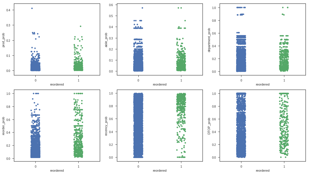
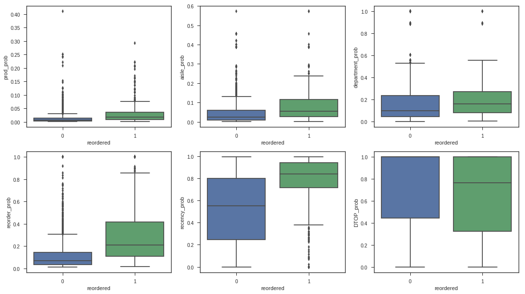
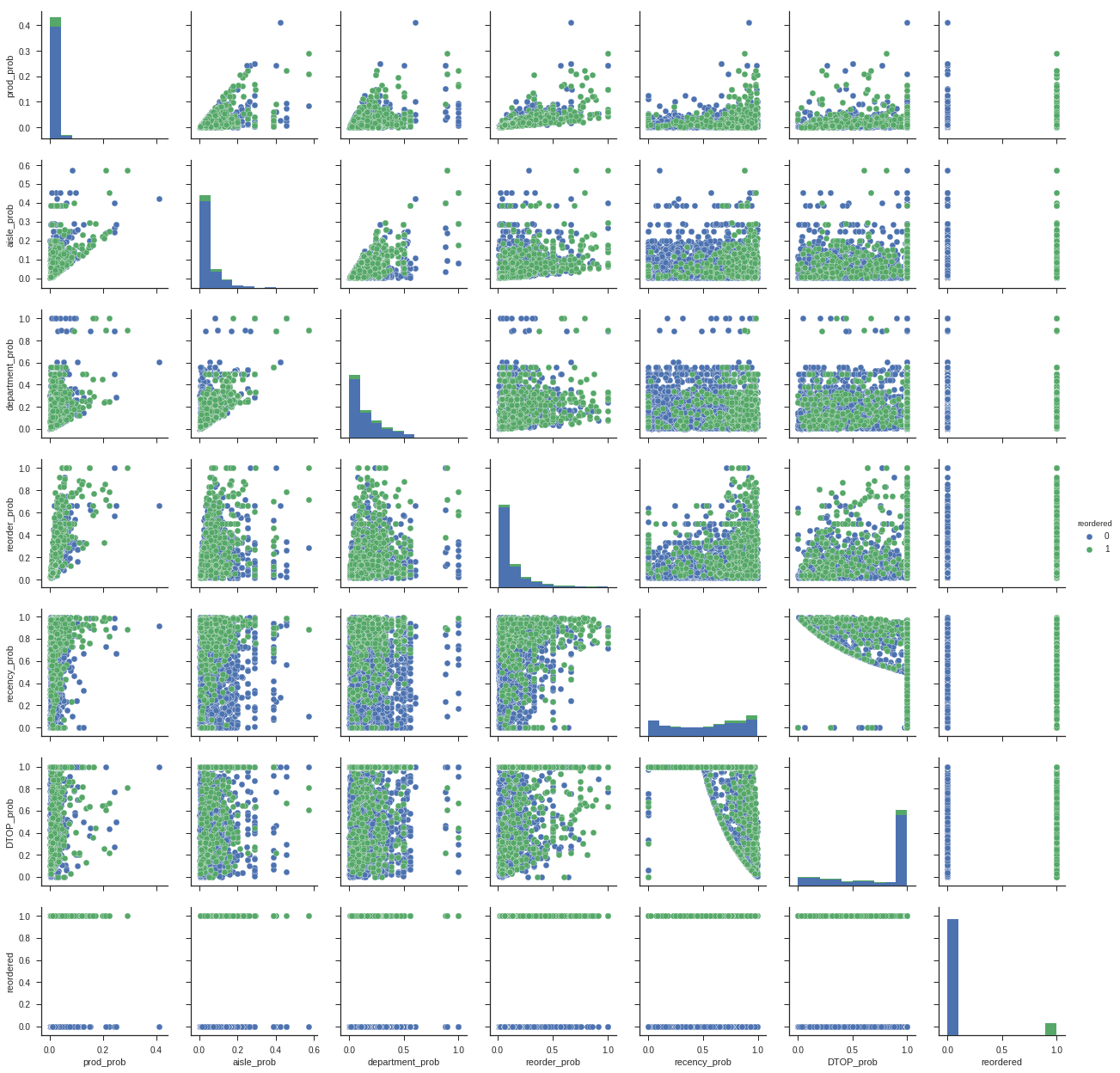
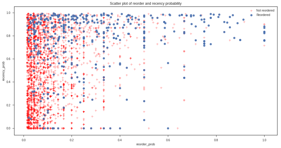
We will now build and evaluate using cross-validation and parameter searching three models using only the two most promising features, reorder probability and recency probability. These features were selected based on the difference in distribution between the products that were reordered and those that were not, as visible in the relevant box plots above.
from sklearn.model_selection import train_test_split
from sklearn.model_selection import RandomizedSearchCV
from sklearn.metrics import f1_score
from sklearn.metrics import accuracy_score
from sklearn.metrics import make_scorer
from sklearn.tree import DecisionTreeClassifier
from sklearn.ensemble import RandomForestClassifier
from sklearn.ensemble import GradientBoostingClassifier
load_first = 50000
seed = 7

X = training_data.loc[:load_first,['reorder_prob','recency_prob']].as_matrix()
y = training_data.loc[:load_first,'reordered'].as_matrix()

X_train, X_test, y_train, y_test = train_test_split(X, y, test_size=0.2, stratify=y, random_state=seed)
Classifiers
def tryClassifier(clf, X_train, X_test, y_train, y_test):
    clf.fit(X_train, y_train)
    y_hat = clf.predict(X_test)
    printmd("F1 score: **{0:.2f}**".format(f1_score(y_test, y_hat)))
    printmd("Accuracy: **{0:.2f}**".format(accuracy_score(y_test, y_hat)))

def tryClassifierProbThresholds(clf, X_test, y_test, startProb=0.2, endProb=1.0, incrementProb=0.1):
    y_hat_probs = clf.predict_proba(X_test)

    best_threshold_prob = 0
    best_f1_score = 0
    for threshold in np.arange(startProb, endProb, incrementProb):
        print("Using {0:.2f} probability threshold for class 1".format(threshold))
        y_hat = (y_hat_probs[:,1] > threshold).astype(int)
        #print(y_hat)
        current_f1_score = f1_score(y_test, y_hat)
        current_accuracy_score = accuracy_score(y_test, y_hat)
        if current_f1_score > best_f1_score:
            best_f1_score = current_f1_score
            best_threshold_prob = threshold
        print("F1: {0:.4f} - Acc: {1:.4f}".format(current_f1_score, current_accuracy_score))
    printmd("Best F1 score: **{0:.4f}** at probability threshold **{1:.2f}**".format(best_f1_score, best_threshold_prob))

printmd("Baseline accuracy if predicting all zeros: ** {0:.2f}% **".format((1 - (np.sum(y_test) / len(y_test)))*100))
Baseline accuracy if predicting all zeros: ** 90.69% **
Decision Tree
clf = DecisionTreeClassifier(random_state=seed, class_weight="balanced")
tryClassifier(clf, X_train, X_test, y_train, y_test)
F1 score: 0.29
Accuracy: 0.79
tryClassifierProbThresholds(clf, X_test, y_test)
Using 0.20 probability threshold for class 1
F1: 0.2571 - Acc: 0.7498
Using 0.30 probability threshold for class 1
F1: 0.2672 - Acc: 0.7642
Using 0.40 probability threshold for class 1
F1: 0.2748 - Acc: 0.7773
Using 0.50 probability threshold for class 1
F1: 0.2850 - Acc: 0.7943
Using 0.60 probability threshold for class 1
F1: 0.2932 - Acc: 0.8163
Using 0.70 probability threshold for class 1
F1: 0.3000 - Acc: 0.8348
Using 0.80 probability threshold for class 1
F1: 0.3046 - Acc: 0.8594
Using 0.90 probability threshold for class 1
F1: 0.2908 - Acc: 0.8717
Best F1 score: 0.3046 at probability threshold 0.80
Random Forest
First we do a randomized parameter search to identify the best hyperparameters for maximum tree depth and number of trees to use.
params = {
    'max_depth': range(2, 30, 2),
    'n_estimators': range(10, 200, 10)
}
clf = RandomForestClassifier(random_state=seed, n_jobs=-1, class_weight="balanced_subsample")
search = RandomizedSearchCV(clf, params, n_iter=5, scoring=make_scorer(f1_score), random_state=seed, cv=5)
search.fit(X_train, y_train)
search.best_params_
{'max_depth': 10, 'n_estimators': 140}
search.best_estimator_
RandomForestClassifier(bootstrap=True, class_weight='balanced_subsample',
            criterion='gini', max_depth=10, max_features='auto',
            max_leaf_nodes=None, min_impurity_split=1e-07,
            min_samples_leaf=1, min_samples_split=2,
            min_weight_fraction_leaf=0.0, n_estimators=140, n_jobs=-1,
            oob_score=False, random_state=7, verbose=0, warm_start=False)
printmd("Best F1 score: **{0:.4f}**".format(search.best_score_))
Best F1 score: 0.3595
Refit best estimator model on training data and evaluate F1 performance using various probability thresholds.
tryClassifierProbThresholds(search.best_estimator_.fit(X_train, y_train), X_test, y_test)
Using 0.20 probability threshold for class 1
F1: 0.2421 - Acc: 0.4510
Using 0.30 probability threshold for class 1
F1: 0.2826 - Acc: 0.5846
Using 0.40 probability threshold for class 1
F1: 0.3395 - Acc: 0.7101
Using 0.50 probability threshold for class 1
F1: 0.3690 - Acc: 0.7787
Using 0.60 probability threshold for class 1
F1: 0.3989 - Acc: 0.8493
Using 0.70 probability threshold for class 1
F1: 0.4024 - Acc: 0.8883
Using 0.80 probability threshold for class 1
F1: 0.3300 - Acc: 0.9074
Using 0.90 probability threshold for class 1
F1: 0.1550 - Acc: 0.9117
Best F1 score: 0.4024 at probability threshold 0.70
Gradient Boosting
params = {
    'learning_rate': np.arange(0.1, 1, 0.1),
    'max_depth': range(2, 30, 2),
    'n_estimators': range(10, 200, 10)
}
clf = GradientBoostingClassifier(random_state=seed)
search = RandomizedSearchCV(clf, params, n_iter=10, scoring=make_scorer(f1_score), random_state=seed, cv=5)
search.fit(X_train, y_train)
search.best_params_
{'learning_rate': 0.5, 'max_depth': 18, 'n_estimators': 50}
search.best_estimator_
GradientBoostingClassifier(criterion='friedman_mse', init=None,
              learning_rate=0.5, loss='deviance', max_depth=18,
              max_features=None, max_leaf_nodes=None,
              min_impurity_split=1e-07, min_samples_leaf=1,
              min_samples_split=2, min_weight_fraction_leaf=0.0,
              n_estimators=50, presort='auto', random_state=7,
              subsample=1.0, verbose=0, warm_start=False)
printmd("Best F1 score: **{0:.4f}**".format(search.best_score_))
Best F1 score: 0.2781
Refit best estimator model on training data and evaluate F1 performance using various probability thresholds.
tryClassifierProbThresholds(search.best_estimator_.fit(X_train, y_train), X_test, y_test)
Using 0.20 probability threshold for class 1
F1: 0.3065 - Acc: 0.8493
Using 0.30 probability threshold for class 1
F1: 0.3071 - Acc: 0.8651
Using 0.40 probability threshold for class 1
F1: 0.2906 - Acc: 0.8760
Using 0.50 probability threshold for class 1
F1: 0.2788 - Acc: 0.8903
Using 0.60 probability threshold for class 1
F1: 0.2661 - Acc: 0.8930
Using 0.70 probability threshold for class 1
F1: 0.2546 - Acc: 0.8958
Using 0.80 probability threshold for class 1
F1: 0.2369 - Acc: 0.8963
Using 0.90 probability threshold for class 1
F1: 0.2252 - Acc: 0.8968
Best F1 score: 0.3071 at probability threshold 0.30
Fitting Random Forest Using All Training Data
clf = RandomForestClassifier(random_state=seed, n_jobs=-1, class_weight="balanced_subsample",
                             max_depth=10, n_estimators=140, verbose=10)
X_train = training_data.loc[:,['reorder_prob','recency_prob']].as_matrix()
y_train = training_data.loc[:,'reordered'].as_matrix()
clf.fit(X_train, y_train)
building tree 1 of 140building tree 2 of 140


[Parallel(n_jobs=-1)]: Done   1 tasks      | elapsed:   19.2s


building tree 3 of 140
building tree 4 of 140
building tree 5 of 140


[Parallel(n_jobs=-1)]: Done   4 tasks      | elapsed:   41.0s


building tree 6 of 140
building tree 7 of 140
building tree 8 of 140
building tree 9 of 140
building tree 10 of 140
building tree 11 of 140


[Parallel(n_jobs=-1)]: Done   9 tasks      | elapsed:  1.6min


building tree 12 of 140
building tree 13 of 140
building tree 14 of 140
building tree 15 of 140
building tree 16 of 140


[Parallel(n_jobs=-1)]: Done  14 tasks      | elapsed:  2.4min


building tree 17 of 140
building tree 18 of 140
building tree 19 of 140
building tree 20 of 140
building tree 21 of 140
building tree 22 of 140
building tree 23 of 140


[Parallel(n_jobs=-1)]: Done  21 tasks      | elapsed:  3.7min


building tree 24 of 140
building tree 25 of 140
building tree 26 of 140
building tree 27 of 140
building tree 28 of 140
building tree 29 of 140
building tree 30 of 140


[Parallel(n_jobs=-1)]: Done  28 tasks      | elapsed:  4.9min


building tree 31 of 140
building tree 32 of 140
building tree 33 of 140
building tree 34 of 140
building tree 35 of 140
building tree 36 of 140
building tree 37 of 140
building tree 38 of 140


[Parallel(n_jobs=-1)]: Done  37 tasks      | elapsed:  6.7min


building tree 39 of 140
building tree 40 of 140
building tree 41 of 140
building tree 42 of 140
building tree 43 of 140
building tree 44 of 140
building tree 45 of 140
building tree 46 of 140
building tree 47 of 140


[Parallel(n_jobs=-1)]: Done  46 tasks      | elapsed:  8.5min


building tree 48 of 140
building tree 49 of 140
building tree 50 of 140
building tree 51 of 140
building tree 52 of 140
building tree 53 of 140
building tree 54 of 140
building tree 55 of 140
building tree 56 of 140
building tree 57 of 140
building tree 58 of 140


[Parallel(n_jobs=-1)]: Done  57 tasks      | elapsed: 10.9min


building tree 59 of 140
building tree 60 of 140
building tree 61 of 140
building tree 62 of 140
building tree 63 of 140
building tree 64 of 140
building tree 65 of 140
building tree 66 of 140
building tree 67 of 140
building tree 68 of 140
building tree 69 of 140


[Parallel(n_jobs=-1)]: Done  68 tasks      | elapsed: 12.8min


building tree 70 of 140
building tree 71 of 140
building tree 72 of 140
building tree 73 of 140
building tree 74 of 140
building tree 75 of 140
building tree 76 of 140
building tree 77 of 140
building tree 78 of 140
building tree 79 of 140
building tree 80 of 140
building tree 81 of 140
building tree 82 of 140


[Parallel(n_jobs=-1)]: Done  81 tasks      | elapsed: 15.4min


building tree 83 of 140
building tree 84 of 140
building tree 85 of 140
building tree 86 of 140
building tree 87 of 140
building tree 88 of 140
building tree 89 of 140
building tree 90 of 140
building tree 91 of 140
building tree 92 of 140
building tree 93 of 140
building tree 94 of 140
building tree 95 of 140


[Parallel(n_jobs=-1)]: Done  94 tasks      | elapsed: 17.5min


building tree 96 of 140
building tree 97 of 140
building tree 98 of 140
building tree 99 of 140
building tree 100 of 140
building tree 101 of 140
building tree 102 of 140
building tree 103 of 140
building tree 104 of 140
building tree 105 of 140
building tree 106 of 140
building tree 107 of 140
building tree 108 of 140
building tree 109 of 140
building tree 110 of 140


[Parallel(n_jobs=-1)]: Done 109 tasks      | elapsed: 20.3min


building tree 111 of 140
building tree 112 of 140
building tree 113 of 140
building tree 114 of 140
building tree 115 of 140
building tree 116 of 140
building tree 117 of 140
building tree 118 of 140
building tree 119 of 140
building tree 120 of 140
building tree 121 of 140
building tree 122 of 140
building tree 123 of 140
building tree 124 of 140
building tree 125 of 140


[Parallel(n_jobs=-1)]: Done 124 tasks      | elapsed: 22.7min


building tree 126 of 140
building tree 127 of 140
building tree 128 of 140
building tree 129 of 140
building tree 130 of 140
building tree 131 of 140
building tree 132 of 140
building tree 133 of 140
building tree 134 of 140
building tree 135 of 140
building tree 136 of 140
building tree 137 of 140
building tree 138 of 140
building tree 139 of 140
building tree 140 of 140


[Parallel(n_jobs=-1)]: Done 140 out of 140 | elapsed: 25.4min finished


RandomForestClassifier(bootstrap=True, class_weight='balanced_subsample',
            criterion='gini', max_depth=10, max_features='auto',
            max_leaf_nodes=None, min_impurity_split=1e-07,
            min_samples_leaf=1, min_samples_split=2,
            min_weight_fraction_leaf=0.0, n_estimators=140, n_jobs=-1,
            oob_score=False, random_state=7, verbose=10, warm_start=False)
Save Random Forest Fitted Model to Disk
from sklearn.externals import joblib
joblib.dump(clf, 'randomforest-all-training-data.pkl')
['randomforest-all-training-data.pkl']


