Analysis of Malta-Sicily Interconnector Usage (2015-2019)
The Malta–Sicily Interconnector connects Malta to the Synchronous grid of Continental Europe through the Ragusa substation in Sicily, operated by the Transmission System Operator - TSO Terna. The interconnector has a power rating of 200MW at 220kV alternating current. The cable was laid by Nexans in 2014 and became fully operational in March 2015. On the 23rd of December 2019 the interconnector was damaged by a ship’s anchor severing the electrical connection. This has deprived Malta of 200MW of on-demand power for the next several months until the cable is fully repaired.
Enemalta, Malta’s electricity service provider, has since switched on all emergency capacity turbines as spinning reserve, at a cost of €150,000 daily, to reduce interruptions in the supply of electricity.
In view of this, we analysed how the interconnector has been used over its initial five years to assess its importance in the supply of energy for Malta’s requirements.
Energy Generation in Malta
This report is focused on the interconnector usage between 2015 and 2019, and so only the power generation facilities available during this period are listed below.
Marsa Power Station
The Marsa power station could generate ~270MW of power and used heavy fuel oil (HFO). This power station was decommissioned on 9th March 2015 and was fully disconnected on 12th March 2017, however, a gas turbine generating 35MW was kept for emergency capacity.
Delimara 1 Power Station
The Delimara 1 power station could generate ~120MW of power and used HFO. This power station was decommissioned on 24th April 2017.
Delimara 2 Power Station
The Delimara 2 power station is composed of D2A and D2B and can generate ~155MW of power using gas oil. This power station was kept on standby for emergency capacity.
Delimara 3 / BWSC / Shanghai Electric
The Delimare 3 power station can generate ~153MW of power. This power station was converted to use Liquefied Natural Gas (LNG) instead of HFO in two phases between May 2016 and August 2017. On 24th April 2017, the first four engines were generating power using LNG.
Delimara 4 / Electrogas
The Delimara 4 power station operates on LNG and can generate ~210MW of power. This power station became operational on 24th April 2017.
Interconnector
The interconnector can provide up to 200MW of electricity and became operational in March 2015, officially being inaugurated on 9th April 2015.
Photovoltaics / Renewable Energy Sources
Enemalta states that 100MW of energy can be sourced from renewable energy sources during ideal periods, however, the average is 95MW. Since most renewable energy in Malta comes from photovoltaic panels, ~95% in 2018, power can only be sourced during daylight.
The above information was collated from the following sources:
- Enemalta Corporation - History of Electricity
- Enemalta Corporation - Delimare Power Station
- Enemalta Corporation - Electricity Generation Plan - 2006 – 2015
- ERA - Delimara Gas and Power - Project Description Statement
- ERA - Marsa Power Station - Decommissioning, Dismantling & Demolition - Project Description Statement
- LovinMalta.com - Interconnector Out Of Action Till At Least February As Faults In Malta’s Power Stations Cause Regular Blackouts
- NSO - Electricity Supply: 2014-2018
- TimesofMalta.com - BWSC plant generated 28 per cent of electricity last year
- TimesofMalta.com - Enemalta: three times the power
- TimesofMalta.com - Malta’s power link to Sicily could be out of action for months after damage
- Wartsila - Malta prepares for an LNG-powered future
Significant Changes in Electricity Generation Capacity
March 2015
On 9th March 2015 the Marsa power station was decommissioned but left on cold standby. During this year, electricity was generated as follows:
| Power Station | Percentage |
|---|---|
| Interconnector | 47% |
| D3 / BWSC | 28% |
| D1 | 18% |
| D2 | 2% |
| Other | 5% |
Source: TimesofMalta.com - BWSC plant generated 28 per cent of electricity last year
The interconnector thus enabled the shutdown of the Marsa Power Station to go ahead. It also reduced emissions by making it possible to not have to rely completely on the Delimara power stations.
9 April 2015
The 200MW rated interconnecter became fully operational during March 2015. Following extensive testing during March, it was officially inaugurated on 9 April 2015.
May 2016 - April 2017
From May 2016 to February 2017, the first phase of converting the Delimara 3 power station from HFO to LNG started. This meant that four out of the eight engines were taken offline, resulting in a loss of ~70MW of power generation. At this point in time Delimara 4 power station was still not generating electricity. Therefore, only D1, D2 and half of D3 could generate power.
Source: Malta prepares for an LNG-powered future
Since D2 runs on gas oil and the amount stored is limited this is not feasible to run for continuous generation.
Source: TimesofMalta.com - Enemalta: three times the power
The interconnector therefore made the D3 power station HFO to LNG conversion project possible since 68% of Malta’s energy requirements for the year 2016, were provided through it.
Source: Electricity from Sicily was main power source last year
24 April 2017
On this day, the Delimara 1 power station was decommissioned and the new LNG powered Delimara 4 went into operation.
Delimara 3 was switched over to the four newly converted dual fuel engines running on LNG. The remaining four HFO engines in Delimara 3 were switched off to undergo conversion to single fuel LNG powered, to be completed by August 2017.
Source: Malta prepares for an LNG-powered future
From this date, Malta could get its electricity from D2, half of D3 till end of August 2017, D4 and the interconnector. D2 is to be used in emergency scenarios, so we can exclude it for normal day to day electricity generation. Theoretically, half of D3 and D4 can generate ~270MW. According to the Malta National Statistics Office (NSO), during 2017 the highest annual average demand was 386MW. During April and May 2017, spring months typically characterised by mild temperatures when electricty demand is usually the lowest throughout the year, the average peak demand was 310MW.
Source: NSO - Electricity Supply: 2014-2018
This means that half of D3 and D4 power stations cannot generate enough electricity to meet the average peak demand for April and May by ~40MW and the highest annual average demand by ~116MW. If the D3 power station is fully operational, following the conversion of the remaining four engines to LNG, it still would not be able to generate enough electricity along with the D4 power station to meet the highest annual average demand of 386MW, falling short by ~26MW.
Under the current circumstances, with both Marsa and D1 power stations decommissioned, the interconnector is clearly essential alongside D3 and D4 to meet the energy requirements of Malta. This becomes more evident when one considers that the above figures are only theoretical. In practice, power station engines experience downtime for maintenance or repair and power generation efficiency changes under different operating conditions, for example, due to seasonal changes in temperature.
Although renewable energy sources are increasing these only represent a small fraction of electricity supplied, ~7% in 2017. Furthermore, most of the renewable energy currently comes from photovoltaic panels, ~95% in 2018. These can only generate power during daylight and their total output decreases significantly when comparing summer and winter months, due to the changes in the sun’s angle of incidence. For instance, during 2018 the electricity produced from renewable energy sources was 10,104MWh in February, while in June it peaked at 22,216MWh.
The percentage of electricity supplied from renewable energy sources has been increasing by ~1% per year and in 2018 stood at 7.8%.
Source: NSO - Electricity Supply: 2014-2018
23 December 2019
On this day, the interconnector cable was severely damaged by an anchor at around 7.30am. Since then Malta has lost 200MW of on-demand power. In the hour before the interconnector cable was damaged, from 6.00am to 6.59am, Malta imported 186MWh of electricity. Enemalta had stated that the interconnector was being used nearly at full capacity at the time of the incident due to “limitations in the capacity of the generating plants in Delimara”. No explanation was given for these limitations.
Source: Enemalta warns of unplanned power cuts after interconnector is damaged at sea
However, once more it becomes clear that the interconnector is crucial both when local power generation is limited for some reason and when all power stations are functioning. In fact, since the interconnector is not available Enemalta has to run the gas oil powered engines in D2 as spinning reserve, at a cost of €150,000 daily. This to reduce interruptions in the supply of electricity.
Furthermore, the interconnector is listed as one of three backup reserve capacity sources, along D2 and the four dual fuel engines of D3, in case there is a shortage of LNG.
Data Visualisations
In this section of the report we will visualise and explore three data sets, namely:
- Peak Monthly Electricity Demand in Malta (2015-2018)
- Hourly Physical Foreign Exchange of Electricity between Malta and Sicily (2015-2019)
- Nitrogen Oxides Emissions from Delimara 4 (Electrogas) Power Station (2017-2019)
The data will be interpreted within the context outlined in the previous two sections, i.e., electricity sources available in Malta and the significant changes that occurred.
Importing Data Analysis and Visualisation Libraries
import datetime
from dateutil import parser
import numpy as np
import pandas as pd
from pandas.plotting import register_matplotlib_converters
register_matplotlib_converters()
%matplotlib inline
import matplotlib.pyplot as plt
import matplotlib.dates as mdates
import seaborn as sns

# set seaborn defaults
sns.set(rc={'figure.figsize':(11, 4)})
sns.set_palette("Set1")
sns.set_style("whitegrid")

def to_short_month(value, tick_number):
    return datetime.datetime(2000, value + 1, 1).strftime('%b')

def to_short_weekday(value, tick_number):
    weekdays = ['Mon','Tue','Wed','Thu','Fri','Sat','Sun']
    return weekdays[abs(value) % len(weekdays)]

def plot_time_series(data_set, plot_labels, chart_title, y_label, start_date, end_date):
    '''
    Plots a line graph of the time series data between start_date and end_date.

    data_set: A pandas dataframe

    plot_labels: A list of columns present in the dataframe to plot

    chart_title: Title to display on top of the chart

    y_label: Label for the y-axis

    start_date: Specify in YYYY-MM-DD HH:MM format
    end_date: Specify in YYYY-MM-DD HH:MM format

    Dates can be as specific as you need, so you can just specify year and month only, for instance.

    Examples:

    Plot data for October and November 2019 inclusive:
    plot_IC_hourly('2019-10', '2019-11')

    Plot data from 14 Oct 2019 to 18 Oct 2019 inclusive:
    plot_IC_hourly('2019-10-14', '2019-10-18')

    Plot data from 10am to 1pm on the 14 Oct 2019:
    plot_IC_hourly('2019-10-14 10:00', '2019-10-14 13:00')
    '''

    if end_date < start_date:
        print('start_date must be before end_date.')
        return

    start = parser.parse(start_date)
    end = parser.parse(end_date)
    diff = end - start

    fig = plt.figure(figsize=(14,4))
    ax = plt.axes()
    plt.grid(b=True, which='minor', color='0.8', linestyle=':', axis='x')
    plt.title('%s [%s to %s]' % (chart_title, start_date, end_date))
    plt.ylabel(y_label)
    for plot_label in plot_labels:
        plt.plot(data_set.loc[start_date:end_date, plot_label],
                 label=plot_label, marker='.', linestyle='-')
    plt.legend()

    if diff.days < 1:
        ax.xaxis.set_major_locator(mdates.DayLocator())
        ax.xaxis.set_major_formatter(mdates.DateFormatter('%d %b %Y'))
        ax.xaxis.set_minor_locator(mdates.HourLocator((0,6,12,18)))
        ax.xaxis.set_minor_formatter(mdates.DateFormatter('%H:%M'))
    elif diff.days < 4:
        ax.xaxis.set_major_locator(mdates.DayLocator(interval=2))
        ax.xaxis.set_major_formatter(mdates.DateFormatter('%d %b %Y'))
        ax.xaxis.set_minor_locator(mdates.HourLocator((0,6,12,18)))
        ax.xaxis.set_minor_formatter(mdates.DateFormatter('%H:%M'))
    elif diff.days < 14:
        ax.xaxis.set_major_locator(mdates.DayLocator(interval=2))
        ax.xaxis.set_major_formatter(mdates.DateFormatter('%d %b %Y'))
    elif diff.days < 28:
        ax.xaxis.set_major_locator(mdates.DayLocator(interval=3))
        ax.xaxis.set_major_formatter(mdates.DateFormatter('%d %b %Y'))
    elif diff.days < 90:
        ax.xaxis.set_major_locator(mdates.MonthLocator())
        ax.xaxis.set_major_formatter(mdates.DateFormatter('%b %Y'))
        ax.xaxis.set_minor_locator(mdates.DayLocator((5,10,15,20,25)))
        ax.xaxis.set_minor_formatter(mdates.DateFormatter('%-d'))
    elif diff.days < 550:
        ax.xaxis.set_major_locator(mdates.YearLocator())
        ax.xaxis.set_major_formatter(mdates.DateFormatter('%Y'))
        ax.xaxis.set_minor_locator(mdates.MonthLocator())
        ax.xaxis.set_minor_formatter(mdates.DateFormatter('%b'))
    else:
        ax.xaxis.set_major_locator(mdates.YearLocator())
        ax.xaxis.set_major_formatter(mdates.DateFormatter('%Y'))
        ax.xaxis.set_minor_locator(mdates.MonthLocator((1,4,7,10)))
        ax.xaxis.set_minor_formatter(mdates.DateFormatter('%b'))
    plt.show()
Peak Monthly Electricity Demand in Malta (2015-2018)
The data set containing monthly peak electricity demand in Malta between 2015 and 2018 was collated from NSO - Electricity Supply: 2014-2018.
peak_demand_2015_2018 = pd.read_csv('peak-demand-2015-2018.csv')
peak_demand_2015_2018['Date'] = pd.to_datetime(peak_demand_2015_2018['Date'], format='%b-%y')
peak_demand_2015_2018.index = peak_demand_2015_2018['Date']
peak_demand_2015_2018['month'] = peak_demand_2015_2018.index.month
peak_demand_2015_2018['year'] = peak_demand_2015_2018.index.year

plt.figure(figsize=(14,4))
ax = sns.barplot(x="month", y="MW", hue="year", data=peak_demand_2015_2018)
ax.set_ylabel('Peak Electricity Demand (MW)')
ax.set_xlabel('')
ax.set_title('Monthly Peak Electricity Demand in Malta (2015-2018)')
ax.xaxis.set_major_formatter(plt.FuncFormatter(to_short_month))
ax.set_ylim(0, 600)
plt.legend(bbox_to_anchor=(1, 0.5), bbox_transform=plt.gcf().transFigure);
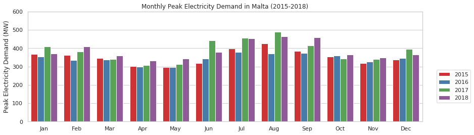
The highest peak summer demand between 2015 and 2018, 488MW, was recorded on 10th August 2017 at 3pm. Data for peak demands for the year 2019 are not available yet, however, Enemalta stated that the peak summer demand for 2019 was 522MW and that on 30th December 2019 demand peaked at 390MW.
Source: TimesofMalta.com - Malta’s power link to Sicily could be out of action for months after damage
# fit a linear equation
y_values = peak_demand_2015_2018['MW']
x_values = np.linspace(0, 1, len(y_values))
coeff = np.polyfit(x_values, y_values, 1)
poly_eq = np.poly1d(coeff)
y_hat = poly_eq(x_values)

# plot peak data and fit data
plt.figure(figsize=(14,4))
ax = plt.axes()
plt.title('Monthly Peak Electricity Demand in Malta (2015-2018)')
plt.ylabel('Peak Electricity Demand (MW)')
plt.ylim(0, 600)
plt.grid(b=True, which='minor', color='0.8', linestyle=':', axis='x')
plt.plot(peak_demand_2015_2018['MW'], marker='.', linestyle='-', label='Peak Demand')
plt.plot(peak_demand_2015_2018['Date'], y_hat, label='Trend')
plt.legend()
ax.xaxis.set_major_locator(mdates.YearLocator())
ax.xaxis.set_major_formatter(mdates.DateFormatter('%Y'))
ax.xaxis.set_minor_locator(mdates.MonthLocator((1,4,7,10)))
ax.xaxis.set_minor_formatter(mdates.DateFormatter('%b'))
plt.show()
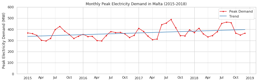
Electricity demand, with the exception of the year 2016, is clearly on an upward trend. For instance, the lowest peak demand in 2018 was registered during April at 331MW, 24MW more than the 307MW peak demand registered in April 2017. Also the peak demand in December 2018 was 366MW, 24MW less than the 390MW registered on 30th December 2019. The highest peak demand was registered in August 2017 at 488MW, but this has been surpassed by 34MW during summer 2019, peaking at 522MW.
Without interconnector the total theoretical electricity generation capacity is of ~533MW. If we derate this capacity by 10% to take into consideration high ambient temperature during summer, that leaves a total of ~480MW, which falls short of peak electricity demands registered during summers. Hopefully, the interconnector will be repaired and fully functional before summer 2020 or rolling blackouts might be required.
Hourly Physical Foreign Exchange of Electricity between Malta and Sicily (2015-2019)
The hourly physical foreign exchange of electricity data set was collected from the Terna website.
Load and Prepare Data
The data was modified so that the values are from the perspective of Malta, instead of Italy, and so the sign of the values in the Net Import column were reversed. Furthermore, columns were renamed accordingly, so Import becomes Export and vice versa.
ic_hourly = pd.read_csv('Terna - Malta IC 2015-2019.csv')
ic_hourly.drop('Country', axis=1, inplace=True)
ic_hourly.rename(index=str, columns={'Import':'Export',
                                     'Export':'Import',
                                     'Physical Foreign Exchange [MW]': 'Net Import'}, inplace=True)
ic_hourly['Net Import'] = -ic_hourly['Net Import']
ic_hourly['Date'] = pd.to_datetime(ic_hourly['Date'], dayfirst=True)

ic_hourly.index = ic_hourly['Date']

ic_hourly['hour'] = ic_hourly.index.hour
ic_hourly['month'] = ic_hourly.index.month
ic_hourly['weekday'] = ic_hourly.index.weekday

years = [str(i) for i in range(ic_hourly['Date'].min().year, ic_hourly['Date'].max().year+1)]
View Data Sample
ic_hourly.loc['2019-12-23']
| Date | Export | Import | Net Import | hour | month | weekday | |
|---|---|---|---|---|---|---|---|
| Date | |||||||
| 2019-12-23 00:00:00 | 2019-12-23 00:00:00 | 0 | 145 | 145 | 0 | 12 | 0 |
| 2019-12-23 01:00:00 | 2019-12-23 01:00:00 | 0 | 132 | 132 | 1 | 12 | 0 |
| 2019-12-23 02:00:00 | 2019-12-23 02:00:00 | 0 | 127 | 127 | 2 | 12 | 0 |
| 2019-12-23 03:00:00 | 2019-12-23 03:00:00 | 0 | 126 | 126 | 3 | 12 | 0 |
| 2019-12-23 04:00:00 | 2019-12-23 04:00:00 | 0 | 132 | 132 | 4 | 12 | 0 |
| 2019-12-23 05:00:00 | 2019-12-23 05:00:00 | 0 | 151 | 151 | 5 | 12 | 0 |
| 2019-12-23 06:00:00 | 2019-12-23 06:00:00 | 0 | 186 | 186 | 6 | 12 | 0 |
| 2019-12-23 07:00:00 | 2019-12-23 07:00:00 | 0 | 88 | 88 | 7 | 12 | 0 |
| 2019-12-23 08:00:00 | 2019-12-23 08:00:00 | 0 | 0 | 0 | 8 | 12 | 0 |
| 2019-12-23 09:00:00 | 2019-12-23 09:00:00 | 0 | 0 | 0 | 9 | 12 | 0 |
| 2019-12-23 10:00:00 | 2019-12-23 10:00:00 | 0 | 0 | 0 | 10 | 12 | 0 |
| 2019-12-23 11:00:00 | 2019-12-23 11:00:00 | 0 | 0 | 0 | 11 | 12 | 0 |
| 2019-12-23 12:00:00 | 2019-12-23 12:00:00 | 0 | 0 | 0 | 12 | 12 | 0 |
| 2019-12-23 13:00:00 | 2019-12-23 13:00:00 | 0 | 0 | 0 | 13 | 12 | 0 |
| 2019-12-23 14:00:00 | 2019-12-23 14:00:00 | 0 | 0 | 0 | 14 | 12 | 0 |
| 2019-12-23 15:00:00 | 2019-12-23 15:00:00 | 0 | 0 | 0 | 15 | 12 | 0 |
| 2019-12-23 16:00:00 | 2019-12-23 16:00:00 | 0 | 0 | 0 | 16 | 12 | 0 |
| 2019-12-23 17:00:00 | 2019-12-23 17:00:00 | 0 | 0 | 0 | 17 | 12 | 0 |
| 2019-12-23 18:00:00 | 2019-12-23 18:00:00 | 0 | 0 | 0 | 18 | 12 | 0 |
| 2019-12-23 19:00:00 | 2019-12-23 19:00:00 | 0 | 0 | 0 | 19 | 12 | 0 |
| 2019-12-23 20:00:00 | 2019-12-23 20:00:00 | 0 | 0 | 0 | 20 | 12 | 0 |
| 2019-12-23 21:00:00 | 2019-12-23 21:00:00 | 0 | 0 | 0 | 21 | 12 | 0 |
| 2019-12-23 22:00:00 | 2019-12-23 22:00:00 | 0 | 0 | 0 | 22 | 12 | 0 |
| 2019-12-23 23:00:00 | 2019-12-23 23:00:00 | 0 | 0 | 0 | 23 | 12 | 0 |
plot_time_series(ic_hourly, ['Net Import'],
                 'Malta - Sicily Interconnector Hourly Net Import',
                 'Electricity (MWh)', '2019-12-22', '2019-12-23')
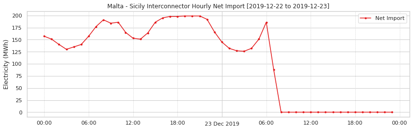
On the 23rd December 2019 at around 7.30am the interconnector was severed. In the figure above it is clear how compared to the previous day, instead of hovering around 180MW till roughly 11am, net electricity import goes down from 186MWh to 88MWh from 6am to 7am and drops to zero as expected under the circumstances.
Maximum MWh Imported
max_elec = ic_hourly['Net Import'].max()
max_elec_date = ic_hourly.loc[ic_hourly['Net Import'] == max_elec]['Date']
print('%d MWh imported on %s' % (max_elec,
                                 max_elec_date[0].strftime('%A, %d %B %Y at %H:%M')))
248 MWh imported on Thursday, 16 August 2018 at 18:00
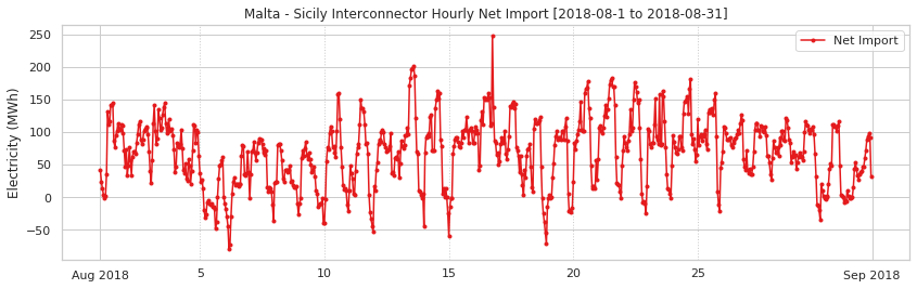
Since the Interconector is rated at 200MW, a peak of 248MWh is interesting. Either this is a data error or the interconnector was being pushed to its limits. The peak demand in August 2018 was:
peak_demand_2015_2018.loc['2018-08']
| Date | MW | month | year | |
|---|---|---|---|---|
| Date | ||||
| 2018-08-01 | 2018-08-01 | 465 | 8 | 2018 |
During August 2018 the interconnector was being used extensively to meet daily peak demands. At this time electricity generation was available through D3 and D4, with D2 as emergency spare capacity. D3 and D4 can theoretically generate ~360MW. Without taking into consideration derating, this stills falls short of the average peaks registered during August. In fact, the interconnector import during daylight fluctuated between 50MWh and 150MWh.
plot_time_series(ic_hourly, ['Net Import'],
                 'Malta - Sicily Interconnector Hourly Net Import',
                 'Electricity (MWh)', '2018-08-1', '2018-08-31')
Maximum MWh Exported
min_elec = ic_hourly['Net Import'].min()
min_elec_date = ic_hourly.loc[ic_hourly['Net Import'] == min_elec]['Date']
print('%d MWh exported on %s' % (min_elec,
                                 min_elec_date[0].strftime('%A, %d %B %Y at %H:%M')))
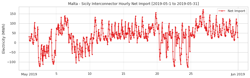
-128 MWh exported on Friday, 24 May 2019 at 13:00
April and May are the months during which electricity demand is the lowest throughout the year, so it is reasonable that the maximum excess electricity generation capacity was available during May 2019.
plot_time_series(ic_hourly, ['Net Import'],
                 'Malta - Sicily Interconnector Hourly Net Import',
                 'Electricity (MWh)', '2019-05-1', '2019-05-31')
Mean Daily Net Import (MWh)
daily_means = ic_hourly[['Export','Import','Net Import','month','weekday']].resample('D').mean()
fig, axes = plt.subplots(len(years), 1, figsize=(18, 25))
plt.subplots_adjust(hspace=0.4)
for year, ax in zip(years, axes):
    ax.plot(daily_means.loc[year, 'Net Import'], label='Net Import', marker='.', linestyle='-')
    ax.plot(daily_means.loc[year, 'Import'], label='Import', marker='.', linestyle='-')
    ax.plot(daily_means.loc[year, 'Export'], label='Export', marker='.', linestyle='-')
    ax.set_title('Malta - Sicily Interconnector Daily Mean Electricity Flow - %s' % year)
    ax.set_ylabel('Electricity (MWh)')
    ax.set_ylim(min(daily_means.loc[year, ['Net Import','Import','Export']].min()-10),
                max(daily_means.loc[year, ['Net Import','Import','Export']].max()+10))
    ax.xaxis.set_major_locator(mdates.MonthLocator())
    ax.xaxis.set_major_formatter(mdates.DateFormatter('%b'))
handles, labels = axes[0].get_legend_handles_labels()
fig.legend(handles, labels, title='', loc='center right')
plt.show()
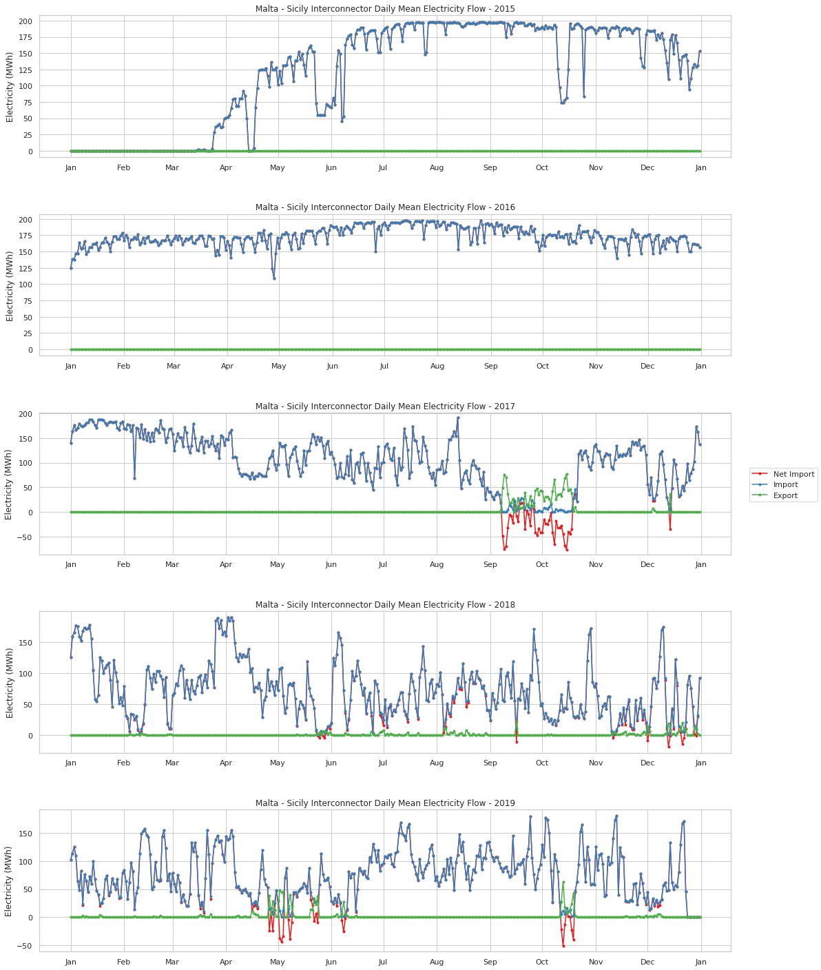
Starting mid-April 2015, the interconnector became a major source of electricity for Malta, being used extensively for the rest of 2015 and nearly at maximum capacity for all of 2016. As discussed this enabled some major changes to be made to Malta’s electricity generation systems, namely, closing down of Marsa power station and conversion of D3 power station from HFO to LNG.
Interconnector usage decreased in 2017 to 2019, compared to 2015 and 2016, however it still hovered around 75MWh on average and on quite a few days still averaged above 150MWh. Past April 2017, D3 and D4 came online, and so there is a lot more variability in usage since the interconnector is supplementing power generation.
Electricity is exported very rarely wih only September and October 2017 and May and October 2019 of particular note. The lowest electricity demands are registered during April, May, September and October. Therefore, excess capacity to export is expected during those months. As for the rest of the year, especially during summer, there is no extra generation capacity to export particularly during day time. Also exporting electricity depends not only on extra capacity but foreign demand and price. Furthermore, Malta is geographically isolated with regards to the European grid, and so demand can mostly come from Sicily and at most southern Italy. Farther north and it makes economic sense to import electricity from cheaper generation available in France and Germany.
Mean Monthly Net Import
monthly_means = ic_hourly[['Export','Import','Net Import','month']].resample('M').mean()
plt.figure(figsize=(14,4))
ax = plt.axes()
plt.title('Malta - Sicily Interconnector Monthly Mean Electricity Flow')
plt.ylabel('Electricity (MWh)')
plt.ylim(min(monthly_means.loc[:,['Net Import','Import','Export']].min()-10),
         max(monthly_means.loc[:,['Net Import','Import','Export']].max()+10))
plt.plot(monthly_means['Net Import'], label='Net Import', marker='o', linestyle='-')
plt.plot(monthly_means['Import'], label='Import', marker='.', linestyle='-')
plt.plot(monthly_means['Export'], label='Export', marker='.', linestyle='-')
plt.legend()
ax.xaxis.set_major_locator(mdates.YearLocator())
ax.xaxis.set_major_formatter(mdates.DateFormatter('%Y'))
ax.xaxis.set_minor_locator(mdates.MonthLocator((1,4,7,10)))
ax.xaxis.set_minor_formatter(mdates.DateFormatter('%b'))
plt.show()
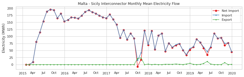
The above plot showing averages for each month clearly shows extensive use of the interconnector during Q3 and Q4 2015, all of 2016 and Q1 2017. From Q2 2017 to end 2018 there is a clear downward trend, however, beginning 2019 interconnector usage is increasing steadily. December 2019’s average is lower since from the 23rd of the month the interconnector is not functioning. The upward trend in interconnector usage during 2019 is in our opinion a sign that the local power generation capacity is not keeping up with the ever increasing demand and so the interconnector has to make up for this gap.
Mean Yearly Net Import
yearly_means = ic_hourly[['Export','Import','Net Import']].resample('Y').mean()
plt.figure(figsize=(14,4))
ax = plt.axes()
plt.title('Malta - Sicily Interconnector Yearly Mean Electricity Flow')
plt.ylabel('Electricity (MWh)')
plt.xlim(datetime.date(2015, 1, 1), datetime.date(2021, 1, 1))
plt.ylim(min(yearly_means.loc[:,['Net Import','Import','Export']].min())-10,
         max(yearly_means.loc[:,['Net Import','Import','Export']].max())+25)
plt.plot(yearly_means['Net Import'], label='Net Import', marker='o', linestyle='-')
plt.plot(yearly_means['Import'], label='Import', marker='.', linestyle='-')
plt.plot(yearly_means['Export'], label='Export', marker='.', linestyle='-')
plt.legend()
yearly_means.apply(lambda r: ax.annotate('%.2f' % r['Net Import'],
                                           (r.name - np.timedelta64('40', 'D'),
                                            r['Net Import']+14))
                   , axis=1);

ax.xaxis.set_major_locator(mdates.YearLocator(month=6, day=30))
ax.xaxis.set_major_formatter(mdates.DateFormatter('%Y'))
plt.show()
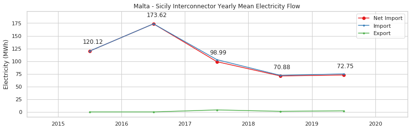
During the years 2018 and 2019, the inteconnector averaged a net import of electricity of 70.88MWh and 72.75Mwh respectively. We are focussing on these years, since past 2017, power generation in Malta has not gone through any significant changes. Both D3 and D4 should be fully functional during this time and therefore it provides a better assessment of how the interconnector is typically used. Next we will plot distributions of the raw hourly data, using box plots, to visualise more clearly the spread of typical usage per period.
Distribution of Net Import per Month
fig, axes = plt.subplots(len(years), 1, figsize=(14, 20))
plt.subplots_adjust(hspace=0.4)
for year, ax in zip(years, axes):
    sns.boxplot(data=ic_hourly.loc[year], x='month', y='Net Import', color='#6495ED', ax=ax)
    ax.set_title('Malta - Sicily Interconnector Distribution of Hourly Net Import per Month - %s' % year)
    ax.set_ylim(ic_hourly.loc[year, 'Net Import'].min()-10,
                ic_hourly.loc[year, 'Net Import'].max()+10)
    ax.set_ylabel('Hourly Net Import (MWh)')
    ax.set_xlabel('')
    ax.xaxis.set_major_formatter(plt.FuncFormatter(to_short_month))
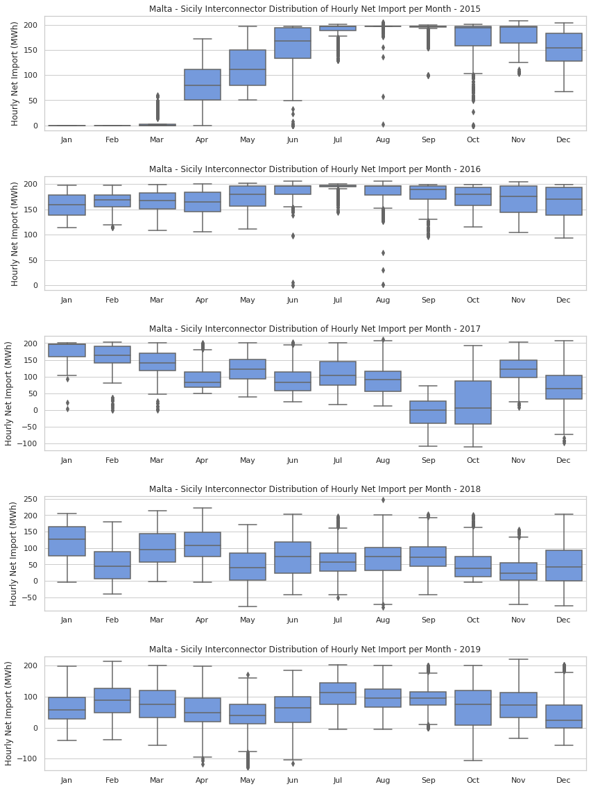
The above distributions show that the interconnector was used extensively during the year 2015 and 2016. In particular, during the whole of 2016, the interconnector was being used to import ~175MWh of power nearly all the time. During July 2016, the distribution is even tighter.
print('July 2017: mean: %.2fMWh std: %.2fMWh' % (
            ic_hourly.loc['2016-07-01':'2016-07-31']['Net Import'].mean(),
            ic_hourly.loc['2016-07-01':'2016-07-31']['Net Import'].std()))
July 2017: mean: 193.31MWh std: 8.85MWh
During 2017, the distributions vary from month to month, however, during September and October there is a clear shift towards exporting electricity. During 2018 and 2019, electricity is for the most part imported, only occasionally being exported. Some seasonality can be observed across the year with some expected higher means during summer, but also some unexpected ones during January, March and April 2018 and February and March 2019. There also seems to be a significant increase in the average electricity imported since July 2019, compared to the first six months of the same year and 2018 overall.
ic_hourly_Qs = ic_hourly['Net Import'].resample('Q')
ic_hourly_Qs_s = pd.concat([ic_hourly_Qs.mean(), ic_hourly_Qs.std()], axis=1)
ic_hourly_Qs_s.columns = ['Mean', 'Std']

plt.figure(figsize=(12,4))
ax = plt.axes()
plt.errorbar(ic_hourly_Qs_s.index,
             ic_hourly_Qs_s.Mean,
             yerr=ic_hourly_Qs_s.Std,
             linestyle='None', marker='o', capsize=3)
ax.set_title('Malta - Sicily Interconnector Mean $\pm$1SD per Quarter (2015 - 2019)')
ax.set_ylabel('Net Import (MWh)')
ax.xaxis.set_major_locator(mdates.YearLocator())
ax.xaxis.set_major_formatter(mdates.DateFormatter('%Y'))
ax.xaxis.set_minor_locator(mdates.MonthLocator((1,4,7,10)))
ax.xaxis.set_minor_formatter(mdates.DateFormatter('%b'))
plt.show()
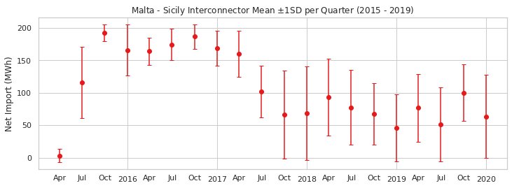
The above plot shows the mean net import in MWh for each quarter in the years 2015 to 2019. Error bars show ±1 standard deviation. From this plot we can confirm that electricity importation increased significantly in Q3 2019 when compared to Q3 2018. The same is also apparent when comparing Q4 2019 to Q4 2018. The increase in Q4 2019 might have been bigger if the interconnector was not severed on 23rd December 2019.
Distribution of Net Import per Day of Week
fig, axes = plt.subplots(len(years), 1, figsize=(14, 20))
plt.subplots_adjust(hspace=0.4)
for year, ax in zip(years, axes):
    sns.boxplot(data=ic_hourly.loc[year], x='weekday', y='Net Import', color='#6495ED', ax=ax)
    ax.set_title('Malta - Sicily Interconnector Distribution of Hourly Net Import per Day of Week - %s' % year)
    ax.set_ylim(ic_hourly.loc[year, 'Net Import'].min()-10,
                ic_hourly.loc[year, 'Net Import'].max()+10)
    ax.set_ylabel('Hourly Net Import (MWh)')
    ax.set_xlabel('')
    ax.xaxis.set_major_formatter(plt.FuncFormatter(to_short_weekday))
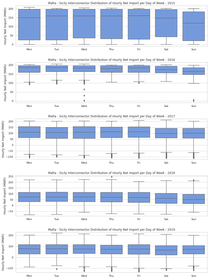
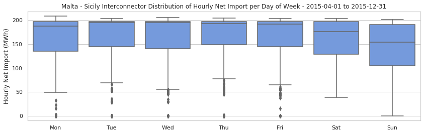
Nothing particular stands out from the above distributions of electricity net import per day of week, except for a minor decrease in use during the weekend. Note that each distribution includes the data for a whole year of that particular week day and if there are any differences across seasons these will not show up.
The distributions for 2015 are a bit too spread out because in the above plot we included the whole year. However, if we plot the distribution for 2015 but exclude the first three months, when the interconnector was not complete or being tested, the interquartile range should be narrower.
fig = plt.figure(figsize=(14, 4))
ax = plt.axes()
sns.boxplot(data=ic_hourly.loc['2015-04-01':'2015-12-31'],
            x='weekday', y='Net Import', color='#6495ED', ax=ax)
ax.set_title('Malta - Sicily Interconnector Distribution of Hourly Net Import per Day of Week - 2015-04-01 to 2015-12-31')
ax.set_ylim(ic_hourly.loc['2015-04-01':'2015-12-31', 'Net Import'].min()-10,
            ic_hourly.loc['2015-04-01':'2015-12-31', 'Net Import'].max()+10)
ax.set_ylabel('Hourly Net Import (MWh)')
ax.set_xlabel('')
ax.xaxis.set_major_formatter(plt.FuncFormatter(to_short_weekday))
Net Import per Hour per Month
In the following figures, we use a strip plot to visualise the net import of electricity during each hour of every month over the last five years. We assigned a dark blue colour for data from midnight to 6.59am and from 7pm to midnight, and an orange colour for data from 7am till 6.59pm. Blue and orange roughly corresponds to the times when the majority of people are inactive or active at work respectively. This is not perfect, since people’s activity changes a lot from winter to summer due to the longer period of daylight time, however, it is tuned to match as much as possible free time (blue) and work time (orange) for the vast majority of people.
colors = ['#053752','#053752','#053752','#053752','#053752','#053752','#053752',
          '#EF810E','#EF810E','#EF810E','#EF810E','#EF810E','#EF810E','#EF810E',
          '#EF810E','#EF810E','#EF810E','#EF810E','#EF810E',
          '#053752','#053752','#053752','#053752','#053752']
sns.set_palette(sns.color_palette(colors))
fig, axes = plt.subplots(len(years), 1, figsize=(14, 20))
plt.subplots_adjust(hspace=0.4)
for year, ax in zip(years, axes):
    sns.stripplot(data=ic_hourly.loc[year], x='month', y='Net Import', hue='hour',
                  jitter=False, dodge=True, alpha=0.5, marker='.', ax=ax)
    ax.set_ylim(ic_hourly.loc[year, 'Net Import'].min()-10,
                ic_hourly.loc[year, 'Net Import'].max()+10)
    ax.set_ylabel('Net Import (MWh)')
    ax.set_title('Malta - Sicily Interconnector Net Import per Hour per Month - %s' % year)
    ax.xaxis.set_major_formatter(plt.FuncFormatter(to_short_month))
    if ax != axes[-1]:
        ax.set_xlabel('')
        ax.get_legend().remove()
    else:
        handles, labels = ax.get_legend_handles_labels()
        fig.legend(handles, labels, title='Hour', loc='right')
        ax.get_legend().remove()
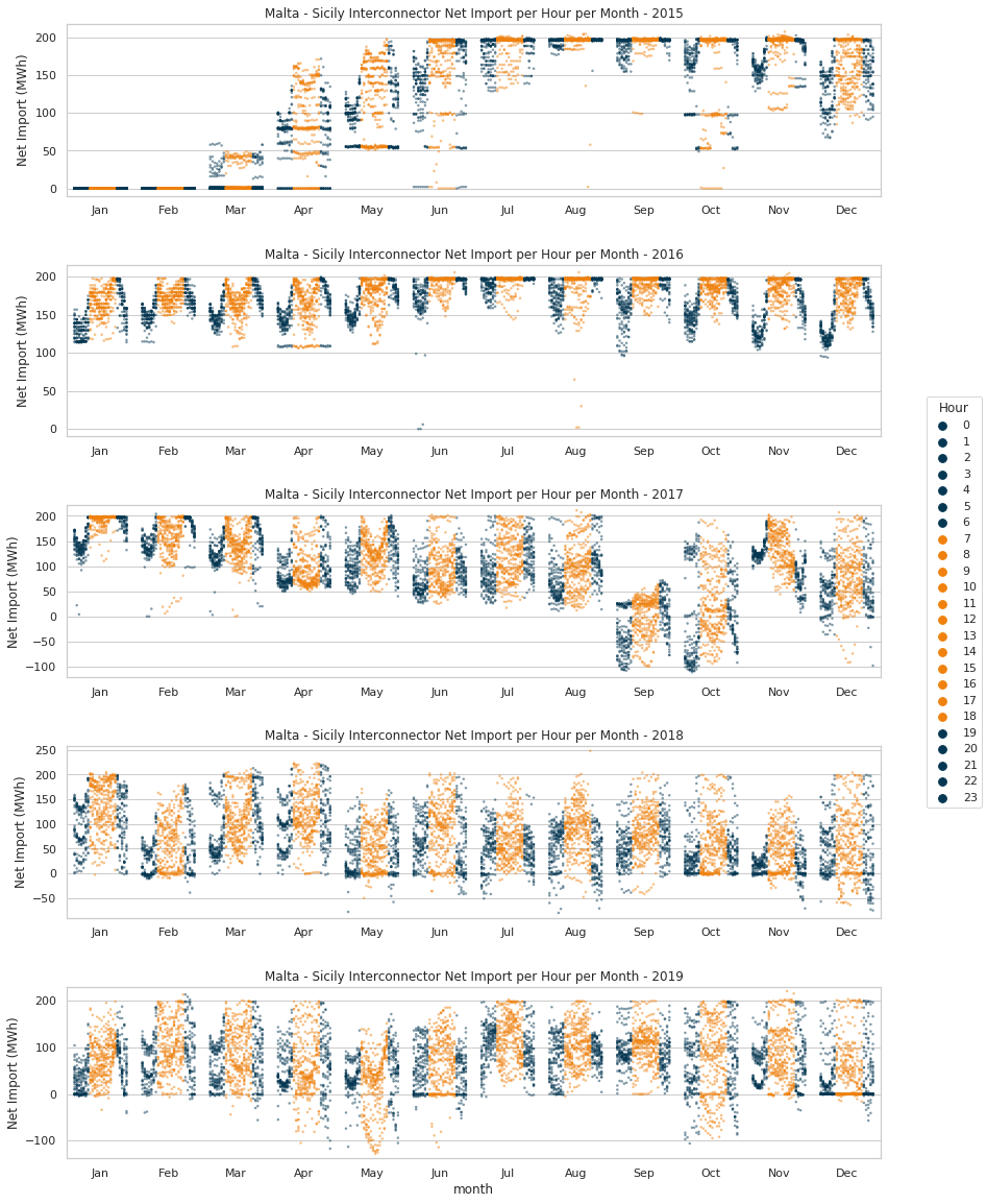
From the above plots it is evident the cyclical nature of interconnector usage throughout each 24-hour period. From troughs around 3am to 5am and noon to 2pm, and peaks around 6am to 9am and 5pm to 8pm. The peaks roughly correspond to when most people wake up and go to work and when they return home. Since this is only data from the interconnector and not the total electricity demand we cannot state definitely that these match the peaks and troughs of the total electricity demand. However, it is highly likely this is the case since the interconnector would be used to meet increased demand.
Nitrogen Oxides Emissions from Delimara 4 (Electrogas) Power Station (2017-2019)
This data set was collated from the Continuous Emissions Monitoring System (CEMS) of Delimara 4 available on CEMS - Electrogas. We only downloaded the nitrogen oxides emissions data since that is the most significant emission of an LNG powered turbine. This should help us determine when each turbine was working. The data downloaded was sorted chronologically and blank values, dashes, were replaced with a zero. We are not sure why there were blanks, possibly sensors or system were not recording, however, we think the simplest explanation is the respective turbine engine was not working at the time.
Loading Data
ccgt_51_hourly = pd.read_csv('sorted-CCGT-51-2017-2019-NO.csv')
ccgt_51_hourly.columns = ['Time', 'NOx - CCGT51']
ccgt_52_hourly = pd.read_csv('sorted-CCGT-52-2017-2019-NO.csv')
ccgt_52_hourly.columns = ['Time', 'NOx - CCGT52']
ccgt_53_hourly = pd.read_csv('sorted-CCGT-53-2017-2019-NO.csv')
ccgt_53_hourly.columns = ['Time', 'NOx - CCGT53']

NOx_emissions = pd.concat([ccgt_51_hourly, ccgt_52_hourly['NOx - CCGT52'], ccgt_53_hourly['NOx - CCGT53']], axis=1)
NOx_emissions['Time'] = pd.to_datetime(NOx_emissions['Time'], dayfirst=True)
NOx_emissions.index = NOx_emissions['Time']

NOx_years = [str(i) for i in range(NOx_emissions['Time'].min().year,
                                    NOx_emissions['Time'].max().year+1)]

NOx_daily_means = NOx_emissions.resample('D').mean()
Mean Daily Nitrogen Oxides Emissions
sns.set_palette('Set1')
fig, axes = plt.subplots(len(NOx_years), 1, figsize=(14, 12))
plt.subplots_adjust(hspace=0.4)
for year, ax in zip(NOx_years, axes):
    ax.set_title('Malta Delimara 4 (Electrogas) Power Station Mean Daily Nitrogen Oxides Emissions - %s' % year)
    ax.set_ylabel('Nitrogen Oxides (MG)')
    ax.set_ylim(min(NOx_daily_means.loc[year].min()-5),
                max(NOx_daily_means.loc[year].max()+10))
    ax.plot(NOx_daily_means.loc[year, 'NOx - CCGT51'], label='NOx - CCGT51', marker='', linestyle='-')
    ax.plot(NOx_daily_means.loc[year, 'NOx - CCGT52'], label='NOx - CCGT52', marker='', linestyle='-')
    ax.plot(NOx_daily_means.loc[year, 'NOx - CCGT53'], label='NOx - CCGT53', marker='', linestyle='-')
    ax.legend(loc='upper right')
    ax.xaxis.set_major_locator(mdates.MonthLocator())
    ax.xaxis.set_major_formatter(mdates.DateFormatter('%b'))
plt.show()
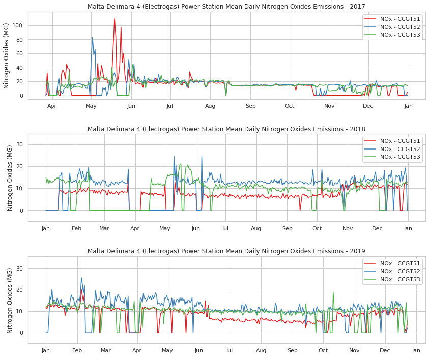
Since we hypothesized that zero emissions is a sign that a turbine is not working, from the above plots we can see that various turbines were not working for quite a number of days. In particular, CCGT51 stands out for the number of days offline and also that overall it seems to be used less intensely than the other turbines. This we can infer from the fact that the emissions of CCGT51 are lower than those of the other two turbines. CCGT53 is also inactive for quite some time, particularly between mid-February and mid-April 2018.
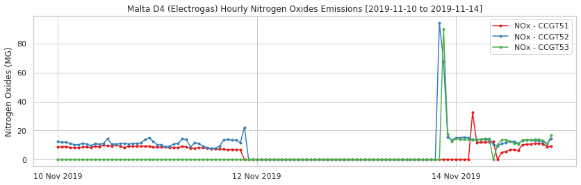
Storm Mooring
From the 11th to the 13th of November 2019, Malta was hit by a storm and the LNG floating storage unit (FSU) tanker was moved some metres away from the jetty. For this reason, LNG gas could not be supplied to the D3 and D4 power stations.
The event was recorded on the Electrogas - Plant Data page as follows:
| Unique Ref Id | Published | Event Start | Event End | Name of Asset | Affected Capacity | Reasons for the Unavailability | Event Status |
|---|---|---|---|---|---|---|---|
| D078 | 11/11/2019 16:49 | 11/11/2019 22:00 | 13/11/2019 10:00 | D4 Plant | 205 MW | Storm Mooring | Dismissed |
| D079 | 13/11/2019 08:40 | 11/11/2019 22:00 | 13/11/2019 22:00 | D4 Plant | 205 MW | Storm Mooring | Inactive |
Based on our hypothesis regarding emissions, we should notice a drop to zero emissions in all turbines at D4 power station. There should also be a corresponding spike in electricity imported through the interconnector to make up for the loss in generation capacity.
plot_time_series(NOx_emissions, ['NOx - CCGT51','NOx - CCGT52','NOx - CCGT53'],
                 'Malta D4 (Electrogas) Hourly Nitrogen Oxides Emissions',
                 'Nitrogen Oxides (MG)', '2019-11-10', '2019-11-14')
plot_time_series(ic_hourly, ['Net Import'],
                 'Malta - Sicily Interconnector Hourly Net Import',
                 'Electricity (MWh)', '2019-11-10', '2019-11-14')
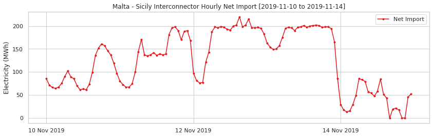
The above plots, show exactly zero emissions from the turbines and a significant increase in the electricity imported through the interconnector during the period while the LNG tanker was moved for storm mooring. This validates our hypothesis that zero emissions is a sign of a turbine which is not working.
Regasification Plant
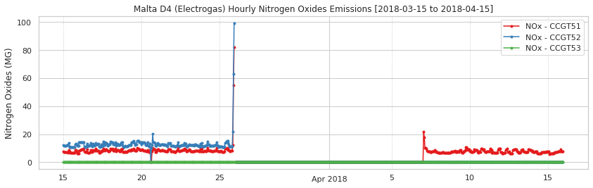
During 2018, from mid-February to mid-April, CCGT53 is offline. During the same period, CCGT51 and CCGT52 also go offline from the last week of March to the first week of April. The Electrogas - Plant Data lists many events between March and June 2018, some planned and others unplanned. The events that seem to match the period when all three turbines stopped working are the following:
| Unique Ref Id | Published | Event Start | Event End | Name of Asset | Affected Capacity | Reasons for the Unavailability | Event Status |
|---|---|---|---|---|---|---|---|
| D002 | 23/03/2018 10:38 | 15/03/2018 10:38 | 04/05/2018 00:00 | D4 Plant | 205 MW | Planned | Dismissed |
| LNG002 | 23/03/2018 10:44 | 26/03/2018 12:00 | 05/04/2018 00:00 | Regas Plant | 19.9 GWh /day | Planned | Inactive |
plot_time_series(NOx_emissions, ['NOx - CCGT51','NOx - CCGT52','NOx - CCGT53'],
                 'Malta D4 (Electrogas) Hourly Nitrogen Oxides Emissions',
                 'Nitrogen Oxides (MG)', '2018-03-15', '2018-04-15')
plot_time_series(ic_hourly, ['Net Import'],
                 'Malta - Sicily Interconnector Hourly Net Import',
                 'Electricity (MWh)', '2018-03-15', '2018-04-15')
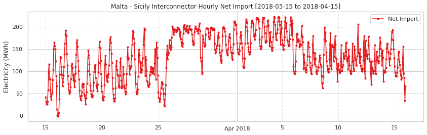
Once more the interconnector fills the gap in electricity generation until the D4 power station turbines are switched back on.
Generation Capacity Under No LNG Supply Scenario
In both the above incidents, the D4 power station could not be supplied with LNG. In the first incident it was because the LNG FSU tanker had to be storm moored away from the jetty. In the second incident, the regasification plant was planned to be unavailable for ten days. Therefore, during both periods the D4 power station was not generating electricity.
Regarding the planned regasification plant unavailability, we do not know why this occurred. Typically, planned downtime would occur for maintenance, but ten days seems a lot. Another possible reason could be transfer of LNG from an LNG tanker to the LNG FSU tanker. Once more, ten days seems too much, unless the LNG tanker was delayed for some reason and the LNG FSU tanker ran out of LNG to supply the power stations.
Furthermore, although we do not have data regarding the D3 power station, we can infer that since it has been converted to LNG, if the LNG supply is unavailable, only four engines can be run using gas oil. Thus, under such scenarios D3 could only generate ~75MW of power.
Therefore, when LNG cannot be supplied, for whichever reason, Malta’s generation capacity is severely limited losing D4 and half of D3, a total of ~285MW. This leaves, ~75MW from D3, ~155MW from D2 and ~35MW from Marsa for a nominal total of ~265MW all running on gas oil. The interconnector adds 200MW taking the total to ~465MW.
The logical choice, from most aspects, is to fill the majority of this gap in generation capacity using the interconnector. Firstly, because the Marsa and D2 generation systems are old and not as efficient as D3 or the interconnector. Secondly, there is only a limited supply of gas oil on land and so D2 and Marsa should only be used in emergency scenarios. In fact, in both scenarios investigated above, the interconnector was used extensively.
Under the present situation, with the interconnector severed, if an LNG shortage had to reoccur we think Malta would not be able to meet its energy requirements reliably based on the above calculations.
Downtime per D4 Power Station Turbine
Since the emissions data is per hour and per turbine we can calculate the percentage of time per year that each turbine was unavailable. We can also compute the annual D4 power station downtime percentage by combining the time from all three turbines.
downtime = {'Year':[],'CCGT51':[],'CCGT52':[],'CCGT53':[],'D4 Total':[]}
for NOx_year in NOx_years:
    NOx_year_emissions = NOx_emissions.loc[NOx_year]
    total_hours = len(NOx_year_emissions)
    CCGT51_zero_NOx = len(NOx_year_emissions[NOx_year_emissions['NOx - CCGT51'] == 0])
    CCGT52_zero_NOx = len(NOx_year_emissions[NOx_year_emissions['NOx - CCGT52'] == 0])
    CCGT53_zero_NOx = len(NOx_year_emissions[NOx_year_emissions['NOx - CCGT53'] == 0])

    CCGT51_per = (CCGT51_zero_NOx/total_hours)*100
    CCGT52_per = (CCGT52_zero_NOx/total_hours)*100
    CCGT53_per = (CCGT53_zero_NOx/total_hours)*100
    D4_total_perc = (CCGT51_zero_NOx + CCGT52_zero_NOx + CCGT53_zero_NOx) / (total_hours*3) * 100

    downtime['Year'].extend([NOx_year])
    downtime['CCGT51'].extend([CCGT51_per])
    downtime['CCGT52'].extend([CCGT52_per])
    downtime['CCGT53'].extend([CCGT53_per])
    downtime['D4 Total'].extend([D4_total_perc])

downtime_df = pd.DataFrame(downtime)
downtime_df_melted = downtime_df.melt(id_vars=['Year'])

plt.figure(figsize=(14,4))
ax = sns.barplot(x="Year", y="value", hue="variable", data=downtime_df_melted)
ax.set_ylabel('Downtime (%)')
ax.set_xlabel('')
ax.set_title('Malta D4 (Electrogas) Power Station Downtime Percentage (2017-2019)')
ax.set_ylim(0, 100)
plt.legend(bbox_to_anchor=(1, 0.5), bbox_transform=plt.gcf().transFigure);
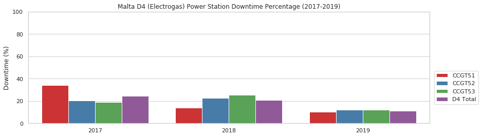
The downtime for each turbine goes down dramactically in 2019 to ~11%. CCGT51 had ~34% and ~14% of downtime in 2017 and 2018 respectively. CCGT52 and CCGT53 hovered around 20% downtime during 2017 and 2018. These reductions in downtime could be due to many factors. At the end of 2017, Enemalta made reference to some issues in an interview, ‘Unreliability and faults’ found at new Electrogas power plant, that were in a later interview, Power station gas tanker refilled eight times this year, said to have been resolved. This could explain the reduction in downtime, especially for CCGT51.
Distribution of Hourly Nitrogen Oxides Emissions
From the mean daily nitrogen oxides emissions plots, found at the beginning of this section, we notice that emissions decrease for all turbines from 2017 to 2019. Decreased emissions could be a result of improved technology or a cleaner LNG supply.
However, it could also correlate to a reduction in turbine engine use. We do not have hourly power generation data for each turbine at D4, so we cannot reach specific conclusions or verify our hypothesis.
To visualise this reduction in emissions better, we plot the distribution of emissions of each turbine per year. So as not to skew the data we eliminated zero emissions, i.e. when a turbine is not working. Furthermore, we do not plot outliers and use the same limits on the y-axis across years to make visual comparison easier.
fig, axes = plt.subplots(len(NOx_years), 1, figsize=(14, 12))
plt.subplots_adjust(hspace=0.4)
for NOx_year, ax in zip(NOx_years, axes):
    NOx_emissions_melted = NOx_emissions.loc[NOx_year].melt(id_vars=['Time'],
                                                            value_vars=['NOx - CCGT51',
                                                                        'NOx - CCGT52',
                                                                        'NOx - CCGT53'])
    NOx_emissions_melted_not_zero = NOx_emissions_melted[NOx_emissions_melted.value > 0]
    sns.boxplot(data=NOx_emissions_melted_not_zero,
                x='variable', y='value',
                showfliers=False, ax=ax)
    ax.set_title('Malta D4 (Electrogas) Power Station Nitrogen Oxides Emissions - %s' % NOx_year)
    ax.set_ylim(0, 40)
    ax.set_ylabel('Nitrogen Oxides (MG)')
    ax.set_xlabel('')
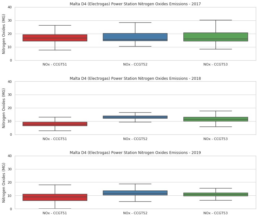
The box plots confirm that the emissions decreased for all three turbines when compared to 2017. The reduction in emissions is most marked in CCGT51.
Conclusion
In this report, we assessed the importance of the interconnector in the supply of energy for Malta’s requirements. To do this we first outlined the power generation options available in Malta and documented key changes to its composition. This allowed us to analyse data in its proper context.
Then we analysed three data sets. Firstly, the Peak Monthly Electricity Demand in Malta (2015-2018), to flesh out the electricity market in Malta with peak demands and electricity demand trends. Secondly, we analysed the Hourly Physical Foreign Exchange of Electricity between Malta and Sicily (2015-2019), to accurately assess when and how the interconnector was used. Finally, we analysed the Nitrogen Oxides Emissions from Delimara 4 (Electrogas) Power Station (2017-2019), since D4 is the new LNG power station entrusted to provide the base load. Since we have no hourly data regarding power generation at D4, we used emissions data to infer turbine activity.
Apart from visualising the data within these data sets, we assessed the data within the context of key dates and events, such as, closing down of the Marsa power station, conversion of the D3 power station from HFO to LNG and scenarios when LNG cannot be supplied to the D3 and D4 power stations.
In all of these scenarios the interconnector proved to be indispensable. For instance, during 2016 it provided 68% of Malta’s energy requirements, with an hourly median above 150MWh throughout the year and in July 2016 reaching a median of ~193MWh. This made the closing down of the Marsa power station, conversion of D3 to LNG and completion of D4 possible. During 2017, it also made it possible to close down D1, in view that D3 was still undergoing conversion till August 2017 and D4 was still going through some issues.
When LNG could not be delivered, due to either storm mooring of the LNG FSU tanker or other reasons, the interconnector filled the gap in electricity generation capacity. LNG delivery to the D3 and D4 power stations has become crucial for Malta, especially now that the interconnector is severed. Until the interconnector is repaired, any disruption to LNG delivery would most probably cause blackouts, since the emergency capacity through D2 and four turbines at D3 all running on gasoil would in all likelihood not meet the electricity demand.
Even under normal circumstances, with D3, D4 and the interconnector fully operational, in view of the ever increasing electricity demand as evidenced by the peaks reached in summer 2019 of 522MW and that on 30th December 2019 of 390MW, the interconnector remains a vital part of Malta’s energy options. D3 and D4 on their own can theoretically generate ~360MW, still ~30MW short of the peak reached in December 2019. Enemalta could make use of D2 as well, however, the interconnector is a better option.
Based on this assessment the interconnector was and still remains crucial for Malta to meet its electricity requirements. We can only hope that the interconnector is repaired in the shortest time possible, ideally before summer 2020 starts.